33 Intro to Decision Trees
In this chapter we introduce decision trees, which are one the most visually atractive and intuitive supervised learning methods. In particular, we will focus our discussion around one kind of trees, the CART-style binary decision trees from the methodology developed in the early 1980s by Leo Breiman, Jerome Friedman, Charles Stone, and Richard Olshen. On the downside, we should say that single trees tend to have high variance, and suffer from overfitting. However, when combined in an ensemble of trees (e.g. bagging, random forests)—using clever sampling strategies—they become powerful predicting tools.
33.1 Introduction
Trees are used in classification and regression tasks by detecting a set of rules allowing the analyst to assign the individuals in data into a class or assign it a predicted value.
Here’s an example with iris data set. This data consists of 5 variables measured on \(n = 150\) iris flowers. There are \(p\) = 4 predictors, and one response. The four variables are:
Sepal.LengthSepal.WidthPetal.LengthPetal.Width
The response is a categorical (i.e. qualitative) variables that indicates the species of iris flower with three categories:
setosaversicolorvirginica
Here’s a few rows of iris data:
  Sepal.Length Sepal.Width Petal.Length Petal.Width Species
1          5.1         3.5          1.4         0.2  setosa
2          4.9         3.0          1.4         0.2  setosa
3          4.7         3.2          1.3         0.2  setosa
4          4.6         3.1          1.5         0.2  setosa
5          5.0         3.6          1.4         0.2  setosa
6          5.4         3.9          1.7         0.4  setosa
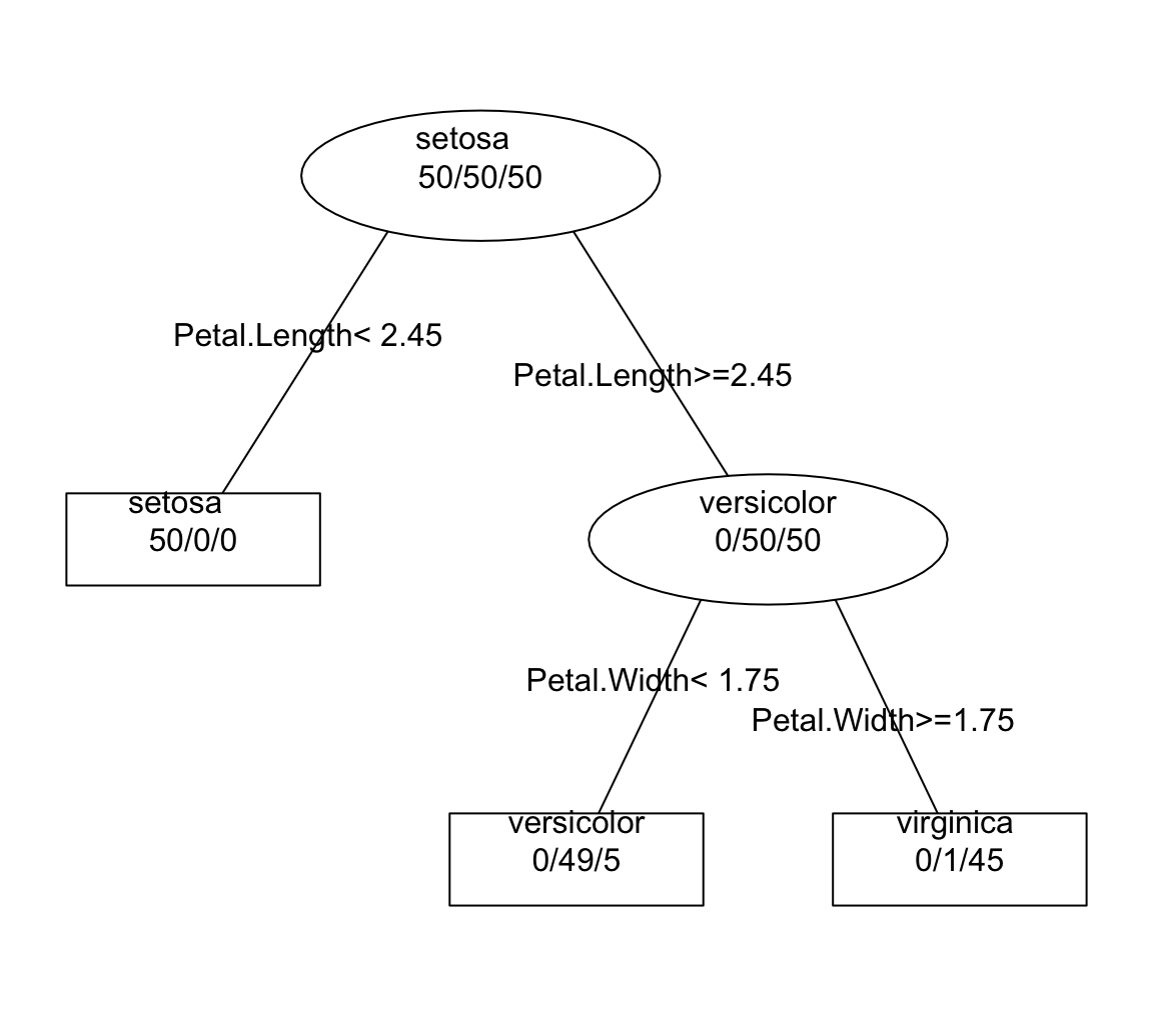
If we use a decision tree to classify the species of iris flowers, we obtain a set of rules can be organized into a hierarchical tree structure. Moreover, this structure can be visually displayed as an inverted tree diagram (although the tree is generally displayed upside down) like in the image below:

Software programs that compute trees, will also return some kind of numeric output like this:
n= 150

node), split, n, loss, yval, (yprob)
      * denotes terminal node

1) root 150 100 setosa (0.33333333 0.33333333 0.33333333)
  2) Petal.Length< 2.45 50   0 setosa (1.00000000 0.00000000 0.00000000) *
  3) Petal.Length>=2.45 100  50 versicolor (0.00000000 0.50000000 0.50000000)
    6) Petal.Width< 1.75 54   5 versicolor (0.00000000 0.90740741 0.09259259) *
    7) Petal.Width>=1.75 46   1 virginica (0.00000000 0.02173913 0.97826087) *
33.2 Some Terminology
Before looking at how decision trees are built, let’s review some of the terminology commonly employed around them. Decision trees have three types of nodes: root, internal, and leaf nodes. These are depicted in the diagram below.
Figure 33.1: Diagram of a tree structure
There is exactly one root node that contains the entire set of elements in the sample; the root node has no incoming branches, and it may have zero, two, or more outgoing branches.
Internal nodes, each of which is hoped to contain as many elements as possible belonging to one class; each internal node has one incoming branch and two (or more) outgoing branches.
Leaf or terminal nodes which, unlike internal nodes, have no outgoing branches.
The root node can be regarded as the starting node. The branches are the lines connecting the nodes. Every node that is preceded by a higher level node is called a “child” node. A node that gives origin to two (or more) child nodes is called a “parent” node. Terminal nodes are nodes without children. The most common way of visually representing a tree is by means of the classical node-link diagram that connects nodes together with line segments.
Figure 33.2: Common elements of a tree diagram
33.2.1 Binary Trees
One special kind of decision trees are binary trees. They are called binary because the nodes are only partitioned in two (see diagram below).
Figure 33.3: Example of a binary tree diagram
33.3 Space Partitions
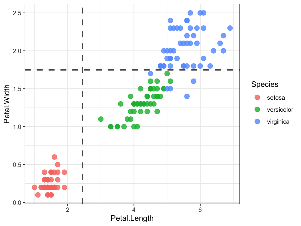
What do partitions of decision trees look like from a geometric standpoint? It turns out that each (binary) split results in a given partition of the feature space. To be more precise, a partition that involves feature \(X_j\) will result in dividing the dimension of \(X_j\) into two regions, depending on the split condition.

In the iris data set example, the first partition is produced by
the condition Petal.Length < 2.45. This condition splits the dimension of
Petal.Length in two regions: a region with petal length values less than 2.45
inches, and another region with petal length values greater than or equal to
2.45 inches. Likewise, the second split is based on the condition
Petal.Width < 1.75, which results in two regions along this dimension.

Toy Abstract Example
Suppose we have two quantitative predictors \(X_1\), and \(X_2\), like in the image below:
Figure 33.4: Two-dimensional feature space
Generally, we create partitions by iteratively splitting one of the predictors into two regions. For example, a first split could be based on \(X_1 = t_1\).
Figure 33.5: First partition
A second split could be produced on a partition for \(X_2\). If \(X_1 \leq t_1\), split on \(X_2 = t_2\). This results in two regions: \(R_1\) and \(R_2\).
Figure 33.6: Second partition
A third split may be detected on the preliminary region \(B\). If \(X_1 > t_1\), split on \(X_3 = t_3\). This results in two regions: \(C\) and \(D\).
Figure 33.7: Third partition
Then, another partition on region \(D\), if \(X_2 = t_4\)
Figure 33.8: Fourth partition
At the end, with a total number of four splits, the feature space is divided in five regions:
Figure 33.9: Regions of feature space
33.3.1 The Process of Building a Tree
Let us begin with the general idea behind binary trees. The main idea is to build a tree structure by successively (i.e. recursively) dividing the set of objects with the help of features \(X_1, \dots, X_p\), in order to obtain the terminal nodes (i.e. final segments) that are as homogeneous as possible (with respect to the response).
The tree building process requires three main components
Establish the set of admissible divisions for each node, that is, compute all possible binary splits.
Define a criterion to find the “best” node split, which requires some criterion to be optimized.
Determine a rule to declare a given node as either internal node, or leaf node.
Establishing the set of admissible splits for each node is related with the nature of the segmentation variables in the data. The number and type of possible binary splits will vary depending on the scale (e.g., binary, nominal, ordinal, and continuous) of the predictor variables. Further discussion is given in the next section.
The second aspect to build a segmentation tree is the definition of a node splitting rule. This rule is necessary to find at each internal node a criterion for splitting the data into subgroups. Since finding a split involves finding the predictor variable that is the most discriminating, the splitting crietroin helps to rank variables according to their discriminating power.
The last component of the tree building process has to do with the definition of a node termination rule. In essence, there are two different ways to deal with this issue: 1) pre-pruning and 2) post-pruning. Pre-pruning implies that the decision of when to stop the growth of a tree is made prospectively. Post-pruning refers to reducing the size of a fully expanded tree by pruning some of its branches retrospectively.