10 Bias-Variance Tradeoff
In this chapter we discuss one of the theoretical dogmas of statistical learning: the famous Bias-Variance tradeoff. Because Bias-Variance (BV) depends on Mean Squared Error (MSE), it is a topic that is typically discussed within the confines of regression, although a generalization is possible to classification problems (but the math is not as clean and straightforward as in regression). Even though we only discuss Bias-Variance from a regression perspective, keep in mind that the practical implications of the bias-variance tradeoff are applicable to all supervised learning contexts.
10.1 Introduction
From the theoretical framework of supervised learning, the main goal is to find a model \(\hat{f}\) that is a good approximation to the target model \(f\), or put it compactly, we want \(\hat{f} \approx f\). By good approximation we mean finding a model \(\hat{f}\) that gives “good” predictions of both types of data points:
- predictions of in-sample data \(\hat{y}_i = \hat{f}(x_i)\), where \((x_i, y_i) \in \mathcal{D}_{in}\)
- and predictions of out-of-sample data \(\hat{y}_0 = \hat{f}(x_0)\), where \((x_0, y_0) \in \mathcal{D}_{out}\)
In turn, these two types of predictions involve two types of errors:
- in-sample error: \(E_{in}(\hat{f})\)
- out-of-sample error: \(E_{out}(\hat{f})\)
Consequently, our desire to have \(\hat{f} \approx f\) can be broken down into two separate wishes that are supposed to be fulfilled simultaneously:
- small in-sample error: \(E_{in}(\hat{f}) \approx 0\)
- out-of-sample error similar to in-sample error: \(E_{out}(\hat{f}) \approx E_{in}(\hat{f})\)
Achieving both wishes essentially means that \(\hat{f}\) is a good model.
Now, before discussing how to get \(E_{out}(\hat{f}) \approx E_{in}(\hat{f})\), we are going to first study some aspects about \(E_{out}(\hat{f})\). More specifically, we are going to study the theoretical behavior of \(E_{out}(\hat{f})\) from a regression perspective, and taking the form of Mean Squared Error (MSE).
10.2 Motivation Example
Let’s start with a toy example. Consider a noiseless target function given by
\[ f(x) = sin(\pi x) \tag{10.1} \]
with the input variable \(x\) in the interval \([-1,1]\), like in the following picture:
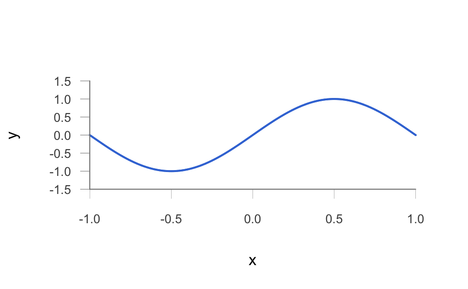
Figure 10.1: Target function
10.2.1 Two Hypotheses
Let’s assume a learning scenario in which, given a data set of \(n\) points, we fit the data using one of two models \(\mathcal{H}_0\) and \(\mathcal{H}_1\) (see the idealized figure shown below):
\(\mathcal{H}_0\): Set of all lines of the form \(h(x) = b\)
\(\mathcal{H}_1\): Set of all lines of the form \(h(x) = b_0 + b_1 x\)
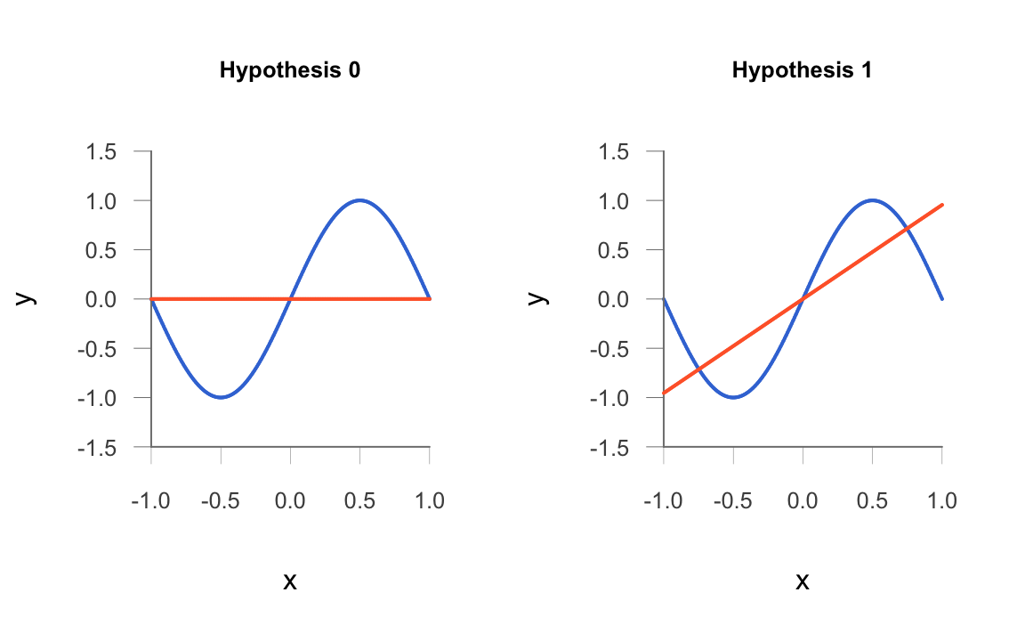
Figure 10.2: Two Learning hypothesis models
10.3 Learning from two points
In this case study, we will assume a tiny data set of size \(n = 2\). That is, we sample \(x\) uniformly in \([-1,1]\) to generate a data set of two points \((x_1, y_1), (x_2, y_2)\); and fit the data using the two models \(\mathcal{H}_0\) and \(\mathcal{H}_1\).
For \(\mathcal{H}_0\), we choose the constant hypothesis that best fits the data: the horizontal line at the midpoint \(b = \frac{y_1 + y_2}{2}\).
For \(\mathcal{H}_1\), we choose the line that passes through the two data points \((x_1, y_1)\) and \((x_2, y_2)\).
Here’s an example in R of two \(x\)-points randomly sampled from a uniform distribution in the interval \([-1,1]\), and their corresponding \(y\)-points:
\(p_1(x_1, y_1) = (0.0949158, 0.2937874)\)
\(p_2(x_2, y_2) = (0.4880941, 0.9993006)\)
With the given points above, the two fitted models are:
\(h_0(x) = 0.646544\)
\(h_1(x) = 0.123472 + 1.794385 \hspace{1mm} x\)
As you can tell, the fitted lines are very different. As expected, \(h_0\) is a constant line (with zero slope), while \(h_1\) has a steep positive slope. Obviously the fitted lines depend on which two points are sampled. As you can imagine, a new sample of two points \((x_1, y_1)\) and \((x_2, y_2)\) would provide different fitted models \(h_0\) and \(h_1\). So let’s see what could happen if we actually repeat this sampling process multiple times.
Small Simulation
Here’s a simulation of the sampling process described above (e.g. repeat it 500 times): we randomly sample two points in the interval \([-1,1]\), and fit both models \(h_0\) and \(h_1\).
The figures which follow show the resulting 500 fits on the same (random) data sets for both methods. We are also displaying the average hypotheses \(\bar{h}_0\) and \(\bar{h}_1\) (colored in red), in each case.
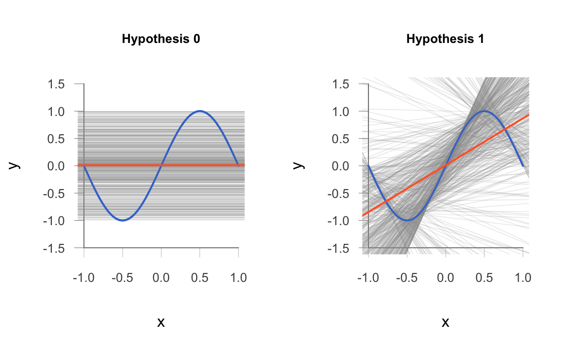
Look at the plot of \(\mathcal{H}_0\) models (the constant lines). If we average all 500 fitted models, we get \(\bar{h}_0\) which roughly corresponds to the horizontal line at \(y = 0\) (i.e. the red horizontal line). Generally speaking, all the individual fitted lines have the same slope of the average hypothesis, but different \(y\)-intercept values. We say that the class of \(\mathcal{H}_0\) models have “low” variance, and “high” bias.
What about the plot of \(\mathcal{H}_1\) models? Averaging all 500 fitted models, we get \(\bar{h}_1\) which roughly corresponds to the red line with positive slope. Generally speaking, the individual fitted lines have all sorts of slopes from extremely negative, to zero or close to zero, to extremely positive. This reflects the fact that there is a substantial amount of variability between the average profile \(\bar{h}_1\) and the form of any single fit \(h_1\). However, the fact that the average hypothesis has positive slope, tells us that the majority of fitted lines also have positive slope. Moreover, the average hypothesis somewhat matches the overall trend of the target function \(f()\) around its middle section (range of \(x \in [-0.5, 0.5]\)). We can summarize all of this by saying that the class of \(\mathcal{H}_1\) models have “high” variance, and “low” bias.
We hope that this simulation example gives you a good starting point to motivate the discussion of the bias-variance tradeoff. But we know it is not enough, and it does not prove anything mathematically. So let’s go ahead and fully disect this mythical bias-variance concept.
10.4 Bias-Variance Derivation
From the previous chapter, we saw that the mean squared error (\(\text{MSE}\)) of an estimator \(\hat{\theta}\) can be decomposed in terms of bias and variance as:
\[ \text{MSE}(\hat{\theta}) = \underbrace{\mathbb{E} [(\hat{\theta} - \mu_{\hat{\theta}})^2]}_{\text{Variance}} + (\underbrace{\mu_{\hat{\theta}} - \theta}_{\text{Bias}})^2 \tag{10.2} \]
with \(\mu_{\hat{\theta}} = \mathbb{E}(\hat{\theta})\). In words:
the bias, \(\mu_{\hat{\theta}} - \theta\), is the tendency of \(\hat{\theta}\) to overestimate or underestimate \(\theta\) over all possible samples.
the variance, \(\text{Var}(\hat{\theta})\), simply measures the average variability of the estimators around their mean \(\mathbb{E}(\hat{\theta})\).
In this chapter, though, we are not talking about any generic estimator \(\hat{\theta}\). In this chapter we are discussing things within the confines of regression. More specifically, the estimator we are dealing with is \(\hat{f}()\), our approximation of a target function \(f()\). Because of this very particular point of view, we need to study the BV decomposition in more detail.
10.4.1 Out-of-Sample Predictions
In order to talk about the mean squared error \(\text{MSE}\) as a theoretical expected value—as opposed to an empirical average—we have to suppose the existance of an out-of-sample data point \(x_0\).
Given a learning data set \(\mathcal{D}\) of \(n\) points, and a hypothesis \(h(x)\), the expectation of the Squared Error for a given out-of-sample point \(x_0\), over all possible learning sets, is expressed as:
\[ \mathbb{E}_{\mathcal{D}} \left [ \left( h^{(\mathcal{D})}(x_0) - f(x_0) \right)^2 \right ] \tag{10.3} \]
For the sake of simplicity, assume the target function \(f()\) is noiseless. Of course this is an idealistic assumption but it will help us to simplify notation. Here, \(h^{(\mathcal{D})}(x_0)\) denotes the predicted value—of an out-of-sample point \(x_0\)—by model \(h()\) fitted on a specific learning data set \(\mathcal{D}\). This is nothing but an estimator, and we can treat \(h^{(\mathcal{D})}(x_0)\) as playing the role of \(\hat{\theta}\). Likewise, \(f(x_0)\) plays the role of \(\theta\).
What about the term that corresponds to \(\mu_{\hat{\theta}} = \mathbb{E}(\hat{\theta})\)? To answer this question we need to introduce a new term:
\[ \bar{h}(x_0) = \mathbb{E}_{\mathcal{D}} \left[ h^{(\mathcal{D})}(x_0) \right] \qquad \text{average hypothesis} \tag{10.4} \]
simply put, think of this term as the average hypothesis.
Now that we have the names and symbols for all the ingredients, let’s do the algebra to find out what the expected squared error for a given out-of-sample point \(x_0\), over all possible learning sets, turns out to be. In order to proceed with the derivation, we need to use a clever trick of adding and subtracting \(\bar{h}\) as follows:
\[ h^{(\mathcal{D})}(x_0) - f(x_0) = h^{(\mathcal{D})}(x_0) - \bar{h}(x_0) + \bar{h}(x_0) - f(x_0) \tag{10.5} \]
To have a less cluttered notation, let’s temporarily “drop” the out-of-sample point \(x_0\). This allows us to simplify the above equation as follows:
\[ h^{(\mathcal{D})} - f = h^{(\mathcal{D})} - \bar{h} + \bar{h} - f \tag{10.6} \]
With these little tricks in mind, here’s the derivation of the expectation:
\[\begin{align*} \mathbb{E}_{\mathcal{D}} \left [ \left( h^{(\mathcal{D})} - f \right)^2 \right ] &= \mathbb{E}_{\mathcal{D}} \left [ \left (h^{(\mathcal{D})} - \bar{h} + \bar{h} - f \right)^2 \right ] \\ &= \mathbb{E}_{\mathcal{D}} \Big [ \Big (\underbrace{h^{(\mathcal{D})} - \bar{h}}_{a} + \underbrace{\bar{h} - f}_{b} \Big)^2 \Big ] \\ &= \mathbb{E}_{\mathcal{D}} \left [ (a + b)^2 \right ] \\ &= \mathbb{E}_{\mathcal{D}} \left [ a^2 + 2ab + b^2 \right ] \\ &= \mathbb{E}_{\mathcal{D}} [a^2] + \mathbb{E}_{\mathcal{D}} [b^2] + \mathbb{E}_{\mathcal{D}} [2ab] \\ \tag{10.7} \end{align*}\]
Let’s examine the first two terms:
\(\mathbb{E}_{\mathcal{D}} [a^2] = \mathbb{E}_{\mathcal{D}} \left [ \left (h^{(\mathcal{D})} - \bar{h} \right)^2 \right ] = \text{Variance} \left( h \right)\)
\(\mathbb{E}_{\mathcal{D}} [b^2] = \mathbb{E}_{\mathcal{D}} \left [ \left (\bar{h} - f \right)^2 \right ] = \text{Bias}^2 \left( h \right)\)
Now, what about the cross-term: \(\mathbb{E}_{\mathcal{D}} [2ab]\)?
\[\begin{align*} \mathbb{E}_{\mathcal{D}} [2ab] & \longrightarrow \mathbb{E}_{\mathcal{D}} \left[ 2 ( h^{(\mathcal{D})} - \bar{h} ) \left( \bar{h} - f \right) \right] \\ &= 2 \mathbb{E}_{\mathcal{D}} \left[ h^{(\mathcal{D})} \bar{h} - h^{(\mathcal{D})} f - \bar{h}^2 + \bar{h} f \right] \\ & \propto \bar{h} \mathbb{E}_{\mathcal{D}}[h^{(\mathcal{D})}] - f\mathbb{E}_{\mathcal{D}}[h^{(\mathcal{D})}] - \mathbb{E}_{\mathcal{D}} [\bar{h}^2] + f \mathbb{E}_{\mathcal{D}} [\bar{h}] \\ &= \bar{h}^2 - f \bar{h} - \bar{h}^2 + f \bar{h} = 0 \tag{10.8} \end{align*}\]
Hence, under the assumption of a noiseless target function \(f\), we have that the expectation of the Squared Error for a given out-of-sample point \(x_0\), over all possible learning sets, is expressed as:
\[\begin{align} \mathbb{E}_{\mathcal{D}} \left [ \left( h^{(\mathcal{D})}(x_0) - f(x_0) \right)^2 \right ] &= \underbrace{\mathbb{E}_{\mathcal{D}} \left [ \left (h^{(\mathcal{D})}(x_0) - \bar{h}(x_0) \right)^2 \right ]}_{\text{variance}} \\ &+ \underbrace{ (\bar{h}(x_0) - f(x_0))^2 }_{\text{bias}^2} \tag{10.9} \end{align}\]
10.4.2 Noisy Target
Now, when there is noise in the data we have that:
\[ y = f(x) + \epsilon \tag{10.10} \]
If \(\epsilon\) is a zero-mean noise random variable with variance \(\sigma^2\), the bias-variance decomposition becomes:
\[ \mathbb{E}_{\mathcal{D}} \left [ \left (h^{(\mathcal{D})}(x_0) - y_0 \right)^2 \right ] = \text{var} + \text{bias}^2 + \sigma^2 \tag{10.11} \]
Notice that the above equation assumes that the squared error corresponds to just one out-of-sample (i.e. test) point \((x_0, y_0) = (x_0, f(x_0))\).
10.4.3 Types of Theoretical MSEs
At this point we need to make an important confession: for better or for worse, there is not just one type of \(\text{MSE}\). The truth is that there are several flavors of theoretical \(\text{MSE}'s\), listed below in no particular order of importance:
\(\mathbb{E}_\mathcal{D} \left[ \left( h^{\mathcal{D}}(x_0) - f(x_0) \right)^2 \right]\)
\(\mathbb{E}_{\mathcal{X}} \left[ \left( h(x_0) - f(x_0) \right)^2 \right]\)
\(\mathbb{E}_{\mathcal{X}} \left[ \mathbb{E}_\mathcal{D} \left\{ \left( h^{\mathcal{D}}(x_0) - f(x_0) \right)^2 \right\} \right]\)
The first MSE involves a single out-of-sample point \(x_0\), measuring the performance of a single type of hypothesis \(h()\) over multiple learning data sets \(\mathcal{D}\). This is what ISL calls expected test MSE (page 34).
The second MSE involves a single hypothesis \(h()\), measuring its performance over all out-of-sample points \(x_0\). Notice that \(h()\) has been fitted on just one learning set \(\mathcal{D}\).
As for the third MSE, this is a combination of the two previous MSEs. Notice how this MSE involves a double expectation. Simply put, it measures the performance of a class of hypothesis \(h()\), over multiple learning data sets \(\mathcal{D}\), over all out-of-sample points \(x_0\). This is what ISL calls overall expected test MSE (page 34).
Unfortunately, in the Machine Learning literature, most authors simply mention an MSE without really specifying which type of MSE. Naturally, this may cause some confusion to the unaware reader. The good news is that, regardless of which MSE flavor you are faced with, they all admit a decomposition into bias-squared, variance, and noise.
We cannot emphasize enough the theoretical nature of any type of \(\text{MSE}\). This means that in practice we will never be able to compute the mean squared error. Why? First, we don’t know the target function \(f\). Second, we don’t have access to all out-of-sample points. And third, we cannot have infinite learning sets in order to compute the average hypothesis. We can, however, try to compute an approximation—an estimate—of an \(\text{MSE}\) using a test data set denoted \(\mathcal{D}_{test}\). This data set will be assumed to be a representative subset (i.e. an unbiased sample) of the out-of-sample data \(\mathcal{D}_{out}\).
10.5 The Tradeoff
We finish this chapter with a brief discussion of the so-called bias-variance (BV) tradeoff. Keep in mind that BV is a good theoretical device; i.e. we can never compute it in practice (if we could, we would have access to \(f\), in which case we wouldn’t really need Statistical Learning in the first place!)
10.5.1 Bias-Variance Tradeoff Picture
Consider several classes of hypothesis, for example a class \(\mathcal{H}_1\) of cubic polynomials; a class \(\mathcal{H}_2\) of quadratic models; and a class \(\mathcal{H}_3\) of linear models. For visualization purposes suppose that we can look at the (abstract) space that contains these types of models, like in the diagram below.

Figure 10.3: An abstract space of hypotheses.
Each hollow (non-filled) point on the diagram above represents a fitted model based on some particular dataset, and each filled point represents the average model of a particular class of hypotheses. For example, if \(\mathcal{H}_1\) represents fits based on linear models, each circle represents some linear polynomial \(ax + b\) with coefficients \(a, b\) that change depending on the sample. We can slightly modify the diagram by grouping all models of the same class, like in the following figure.

Figure 10.4: Space of hypotheses.
Let’s make our diagram more interesting by taking into account the variability in each class of models (see diagram below). In this way, the dashed lines represent the deviations of each fitted model against their average hypothesis. That is, the set of all dashed lines conveys the idea of variance in each model class: i.e. how spread out the models within each class are.

Figure 10.5: Each class of hypothesis has a certain variability.
Finally, suppose that we can also locate the true model in this space, indicated by a solid diammond (see diagram below). Notice that this true model \(f()\) is assumed to be of class \(\mathcal{H}_1\). The solid lines between each average hypothesis and the target function represent the bias of each class of model. In practice, of course, we won’t have access to either the average models (shown in solid colors; i.e. the solid square, triangle, and circle) or the true model (shown in gray).

Figure 10.6: Each class has a certain bias w.r.t. the target function.
Bias
Let’s first focus on the bias, \(\bar{h} - f(x)\). The average \(\bar{h}\) comes from a class of hypotheses (e.g. constant models, linear models, etc.) In other words, \(\bar{h}\) is a prototypical example of a certain class of hypotheses. The bias term thus can be interpreted as a measure of how well a particular type of hypothesis \(\mathcal{H}\) (e.g. constant model, linear model, quadratic model, etc.) approximates the target function \(f\).
Another way to think about bias is as a deterministic noise.
\[ \text{MSE} = \mathrm{Variance} \quad + \underbrace{ \mathrm{Bias}^2 }_{\text{deterministic noise}}+ \underbrace{ \text{Noise} }_{\text{random noise}} \]
Variance
Let’s focus on the variance, \(\mathbb{E}_\mathcal{D} \left[ (h^{(\mathcal{D})}(x) - \bar{h} )^2 \right ]\). This is a measure of how close a particular \(h^{(\mathcal{D})}(x)\) can get to the average functional form \(\bar{h}\). Put it in other terms, how precise is our particular function compared to the average function.
Tradeoff
Ideally, a model should have both small variance and small bias. But, of course, there is a tradeoff between these two (hence the Bias-Variance tradeoff). In general, decreasing bias comes at the cost of increasing variance, and vice-versa.
Also, to understand the bias-variance decomposition, you need access to \(\bar{h}\). In practice, however, we will never have access to \(\bar{h}\) as computing \(\bar{h}\) requires first computing every model of a particular type (e.g. linear, quadratic, etc.).
More complex/flexible models tend to have less bias, and therefore they have a better opportunity to approximate \(f(x)\). They also tend to produce small in-sample error: \(E_{in} \approx 0\).
On the downside, more complex models tend to have higher variance. They also have a higher risk of producing large out-of-sample error: \(E_{out}(h) \neq 0\). You will also need more resources (training data, as well as computational resources) to produce a more complicated model.
Less complex/flexible models (i.e. simpler models) tend to have less variance, but more bias (i.e. less opportunity to estimate \(f\), but a higher chance to approximate out of sample error): \(E_{in} \approx E_{out}\), but \(E_{in} \approx E_{out} \neq 0\). Simpler models also tend to require less data/computational resources.
To decrease bias, a model has to be more flexible/complex. We should note that notions of “flexibility” and “complexity” are difficult to define precisely. For example, in the context of classification, complexity could be related to various hyperparameters (e.g. number of child nodes in our tree, etc.).
In theory, to decrease bias, one needs “insider” information. That is, to truly decrease bias, we need some information on the form of \(f\). Hence, it is nearly impossible to have zero bias. We therefore put our efforts towards decreasing variance when working with more complex/flexible models.
One way to decrease variance would be to add more training data. However, there is a price to pay: we will have less test data.
We could reduce the dimensions of our data (i.e. play with lower-rank data matrices through, for example, PCA).
We could also apply regularization. At its core, this notion relates to making the size of a model’s parameters small. Consequently, there is a reduction in the variance of a model.
In summary: in general, decreasing bias comes at the cost of increasing variance, and vice-versa.