3 Geometric Duality
Before discussing unsupervised as well as supervised learning methods, we prefer to give you a prelude by talking and thinking about data in a geometric sense. This chapter will set the stage for most of the topics covered in later chapters.
Let’s suppose we have some data in the form of a data matrix. For convenience purposes, let’s also suppose that all variables are measured in a real-value scale. Obviously not all data is expressed or even encoded numerically. You may have categorical or symbolic data. But for this illustration, let’s assume that any categorical and symbolic data has already been transformed into a numeric scale (e.g. dummy indicators, optimal scaling).
It’s very enlightening to think of a data matrix as viewed from the glass of Geometry. The key idea is to think of the data in a matrix as elements living in a multidimensional space. Actually, we can regard a data matrix from two apparently different perspectives that, in reality, are intimately connected: the rows perspective and the columns perspective. In order to explain these perspectives, let’s use the following diagram of a data matrix \(\mathbf{X}\) with \(n\) rows and \(p\) columns, with \(x_{ij}\) representing the element in the \(i\)-th row and \(j\)-th column.

Figure 3.1: Duality of a data matrix
When we look at a data matrix from the columns perpective what we are doing is focusing on the \(p\) variables. In a similar way, when looking at a data matrix from its rows perspective, we are focusing on the \(n\) individuals. Like a coin, though, this matrix has two sides: a rows side, and a columns side. That is, we could look at the data from the rows point of view, or the columns point of view. These two views are (of course) not completely independent. This double perspective or duality for short, is like the two sides of the same coin.
3.1 Rows Space
We know that human vision is limited to three-dimensions, but pretend that you had superpowers that let you visualize a space with any number of dimensions.
Because each row of the data matrix has \(p\) elements, we can regard individuals as objects that live in a \(p\)-dimensional space. For visualization purposes, think of each variable as playing the role of a dimension associated to a given axis in this space; likewise, consider each of the \(n\) individuals as being depicted as a point (or particle) in such space, like in the following diagram:

Figure 3.2: Rows space
In the figure above, even though we are showing only three axes, you should pretend that you are visualizing a \(p\)-dimensional space (imaging that there are \(p\) axes). Each point in this space corresponds to a single individual, and they all form what we can call a cloud of points.
3.2 Columns Space
We can do the same visual exercise with the columns of a data matrix. Since each variable has \(n\) elements, we can regard the set of \(p\) variables as objects that live in an \(n\)-dimensional space. However, instead of representing each variable with a dot, it’s better to graphically represent them with an arrow (or vector). Why? Because of two reasons: one is to distinguish them from the individuals (dots). But more important, because the esential thing with a variable is not really its magnitude (and therefore its position) but its direction. Often, as part of the data preprocessing steps, we apply transformations on variables that change their scales (e.g. shrinking them, or stretching them) without modifying their directions. So it’s more convenient to focus primarily on their directions.

Figure 3.3: Columns space
Analogously to the rows space and its cloud of individuals, you should also pretend that the image above is displaying an \(n\)-dimensional space with a bunch of blue arrows pointing in various directions.
What’s next?
Now that we know how to think of data from a geometric perspective, the next step is to discuss a handful of common operations that can be performed with points and vectors that live in some geometric space.
3.3 Cloud of Individuals
In the previous sections, we introduced the powerful idea of looking at the rows and columns of a data matrix from the lens of geometry. We are assuming in general that the rows have to do with \(n\) individuals that lie in a \(p\)-dimensional space.

Figure 3.4: Cloud of points
Let’s start describing a set of common operations that we can apply on the individuals (living in a \(p\)-dimensional space).
3.3.1 Average Individual
We can ask about the typical or average individual.
If you only have one variable, then all the individual points lie in a one-dimensional space, which is basically a line. Here’s a simple example with five individuals described by one variable:

Figure 3.5: Points in one dimension
The most common way to think about the typical or average individual is in terms of the arihmetic average of the values, which geometrically corresponds to the “balancing point”. The diagram below shows three possible locations for a fulcrum (represented as a red triangle). Only the average value 5 results in the balancing point which keeps the values on the number line in equilibrium:

Figure 3.6: Average individual
Algebraically we have: individuals \(x_1, x_2, \dots, x_n\), and the average is:
\[ \bar{x} = \frac{x_1 + \dots + x_n}{n} = \frac{1}{n} \sum_{i=1}^{n} x_i \tag{3.1} \]
In vector notation, the average can be calculated with an inner product between \(\mathbf{x} = (x_1, x_2, \dots, x_n)\), and a constant vector of \(n\)-elements \((1/n)\mathbf{1}\):
\[ \bar{x} = \frac{1}{n} \mathbf{x^\mathsf{T}1} \tag{3.2} \]
What about the multivariate case? It turns out that we can also ask about the average individual of a cloud of points, like in the following figure:

Figure 3.7: Cloud of points with centroid (i.e. average individual)
The average individual, in a \(p\)-dimensional space is the point \(\mathbf{\vec{g}}\) containing as coordiantes the averages of all the variables:
\[ \mathbf{\vec{g}} = (\bar{x}_1, \bar{x}_2, \dots, \bar{x}_p) \tag{3.3} \]
where \(\bar{x}_j\) is the average of the \(j\)-th variable.
This average individual \(\mathbf{\vec{g}}\) is also known as the centroid, barycenter, or center of gravity of the cloud of points.
3.3.2 Centered Data
Often, it is convenient to transform the data in such a way that the centroid of a data set becomes the origin of the cloud of points. Geometrically, this type of transformation involves a shift of the axes in the \(p\)-dimensional space. Algebraically, this transformation corresponds to expressing the values of each variable in terms of deviations from their means.

Figure 3.8: Cloud of points of mean-centered data
In the unidimensional case, say we have \(n\) individuals \(\mathbf{x} = (x_1, x_2, \dots, x_n)\) with a mean of \(\bar{x} = (1/n) \sum_{i=1}^{n} x_i\). The vector of centered values are:
\[ \mathbf{\bar{x}} = (x_1 - \bar{x}, x_2 - \bar{x}, \dots, x_n - \bar{x}) \tag{3.4} \]
In the multidimensional case, the set of centered data values are:
\[ \mathbf{x_1} - \mathbf{g}, \mathbf{x_2} - \mathbf{g}, \dots, \mathbf{x_n} - \mathbf{g} \tag{3.5} \]
3.3.3 Distance between individuals
Another common operation that we may be interested in is the distance between two individuals. Obviously the notion of distance is not unique, since you can choose different types of distance measures. Perhaps the most comon type of distance is the (squared) Euclidean distance. Unless otherwise mentioned, this will be the default distance used in this book.

Figure 3.9: Distance between two individuals
If you have one variable \(X\), then the squared distance \(d^2(i,\ell)\) between two individuals \(x_i\) and \(x_\ell\) is:
\[ d^2(i,\ell) = (x_i - x_\ell)^2 \tag{3.6} \]
In general, with \(p\) variables, the squared distance between the \(i\)-th individual and the \(\ell\)-th individual is:
\[\begin{align*} d^2(i,\ell) &= (x_{i1} - x_{\ell 1})^2 + (x_{i2} - x_{\ell 2})^2 + \dots + (x_{ip} - x_{\ell p})^2 \\ &= (\mathbf{\vec{x}_i} - \mathbf{\vec{x}_\ell})^\mathsf{T} (\mathbf{\vec{x}_i} - \mathbf{\vec{x}_\ell}) \tag{3.7} \end{align*}\]
3.3.4 Distance to the centroid
A special case is the distance between any individual \(i\) and the average individual:
\[\begin{align*} d^2(i,g) &= (x_{i1} - \bar{x}_1)^2 + (x_{i2} - \bar{x}_2)^2 + \dots + (x_{ip} - \bar{x}_p)^2 \\ &= (\mathbf{\vec{x}_i} - \mathbf{\vec{g}})^\mathsf{T} (\mathbf{\vec{x}_i} - \mathbf{\vec{g}}) \tag{3.8} \end{align*}\]
3.3.5 Measures of Dispersion
What else can we calculate with the individuals? Think about it. So far we’ve seen how to calculate the average individual, as well as distances between individuals. The average individual or centroid plays the role of a measure of center. And everytime you get a measure of center, it makes sense to get a measure of spread.
Overall Dispersion
One way to compute a measure of scatter among individuals is to consider all the squared distances between pairs of individuals. For instance, say you have three individuals \(a\), \(b\), and \(c\). We can calculate all pairwise distances and add them up:
\[ d^2(a,a) + d^2(b,b) + d^2(c,c) + \\ d^2(a,b) + d^2(b,a) + \\ d^2(a,c) + d^2(c,a) + \\ d^2(b,c) + d^2(c,b) \tag{3.9} \]
In general, when you have \(n\) individuals, you can obtain up to \(n^2\) squared distances. We will give the generic name of Overall Dispersion to the sum of all squared pairwise distances:
\[ \text{overall dispersion} = \sum_{i=1}^{n} \sum_{\ell=1}^{n} d^2(i,\ell) \tag{3.10} \]
Inertia
Another measure of scatter among individuals can be computed by averaging the distances between all individuals and the centroid.

Figure 3.10: Inertia as a measure of spread around the centroid
The average sum of squared distances from each point to the centroid then becomes
\[ \frac{1}{n} \sum_{i=1}^{n} d^2(i,g) = \frac{1}{n} \sum_{i=1}^{n} (\mathbf{\vec{x}_i} - \mathbf{\vec{g}})^\mathsf{T} (\mathbf{\vec{x}_i} - \mathbf{\vec{g}}) \tag{3.11} \]
We will name this measure Inertia, borrowing this term from the concept of inertia used in mechanics (in physics).
\[ \text{Inertia} = \frac{1}{n} \sum_{i=1}^{n} d^2(i,g) \tag{3.12} \]
What is the motivation behind this measure? Consider the \(p = 1\) case; i.e. when \(\mathbf{X}\) is simply a column vector
\[ \mathbf{X} = \begin{pmatrix} x_1 \\ x_2 \\ \vdots \\ x_n \\ \end{pmatrix} \tag{3.13} \]
The centroid will simply be the mean of these points: i.e. \(\bar{x} = \frac{1}{n} \sum_{i=1}^{n} x_i\).
The sum of squared-distances from each point to the centroid then becomes:
\[ (x_1 - \bar{x})^2 + \dots + (x_n - \bar{x})^2 = \sum_{i=1}^{n} (x_i - \bar{x})^2 \tag{3.14} \]
Does the above formula look familiar? What if we take the average of the squared distances to the centroid?
\[ \frac{1}{n} \sum_{i=1}^{n} (x_i - \bar{x})^2 = \frac{(x_1 - \bar{x})^2 + \dots + (x_n - \bar{x})^2}{n} \tag{3.15} \]
Same question: Do you recognize this formula? You better do… This is nothing else than the formula of the variance of \(X\). And yes, we are dividing by \(n\) (not by \(n-1\)). Hence, you can think of inertia as a multidimensional extension of variance, which gives the typical squared distance around the centroid.
Overall Dispersion and Inertia
Interestingly, the overall dispersion and the inertia are connected through the following relation:
\[\begin{align*} \text{overall dispersion} &= \sum_{i=1}^{n} \sum_{\ell=1}^{n} d^2(i,\ell) \\ &= 2n \sum_{i=1}^{n} d^2(i,g) \\ &= (2n^2) \text{Inertia} \tag{3.16} \end{align*}\]
The proof of this relation is left as a homework exercise.
3.4 Cloud of Variables
The starting point when analyzing variables involves computing various summary measures—such as means, and variances—to get an idea of the common or central values, and the amount of variability of each variable. In this section we will review how concepts like the mean of a variable, the variance, covariance, and correlation, can be interpreted in a geometric sense, as well as their expressions in terms of vector-matrix operations.
3.4.1 Mean of a Variable
To measure variation of one variable, we usually begin by calculating a “typical” value. The idea is to summarize the values of a variable with one or two representative values. You will find this notion under several terms like measures of center, location, central tendency, or centrality.
As mentioned in the previous section, the prototypical summary value of center is the mean, sometimes referred to as average. The mean of an \(n-\)element variable \(X = (x_1, x_2, \dots, x_n)\), represented by \(\bar{x}\), is obtained by adding all the \(x_i\) values and then dividing by their total number \(n\):
\[ \bar{x} = \frac{x_1 + x_2 + \dots + x_n}{n} \tag{3.17} \]
Using summation notation we can express \(\bar{x}\) in a very compact way as:
\[ \bar{x} = \frac{1}{n} \sum_{i = 1}^{n} x_i \tag{3.18} \]
If you associate a constant weight of \(1/n\) to each observation \(x_i\), you can look at the formula of the mean as a weighted sum:
\[ \bar{x} = \frac{1}{n} x_1 + \frac{1}{n} x_2 + \dots + \frac{1}{n} x_n \tag{3.19} \]
This is a slightly different way of looking at the mean that will allow you to generalize the concept of an “average” as a weighted aggregation of information. For example, if we denote the weight of the \(i\)-th individual as \(w_i\), then the average can be expressed as:
\[\begin{align*} \bar{x} &= w_1 x_1 + w_2 x_2 + \dots + w_n x_n \\ &= \sum_{i=1}^{n} w_i x_i \\ &= \mathbf{w^\mathsf{T} x} \tag{3.20} \end{align*}\]
3.4.2 Variance of a Variable
A measure of center such as the mean is not enoguh to summarize the information of a variable. We also need a measure of the amount of variability. Synonym terms are variation, spread, scatter, and dispersion.
Because of its relevance and importance for statistical learning methods, we will focus on one particular measure of spread: the variance (and its square root the standard deviation).
Simply put, the variance is a measure of spread around the mean. The main idea behind the calculation of the variance is to quantify the typical concentration of values around the mean. The way this is done is by averaging the squared deviations from the mean.
\[\begin{align*} Var(X) &= \frac{(x_1 - \bar{x})^2 + \dots + (x_n - \bar{x})^2}{n} \\ &= \frac{1}{n} \sum_{i=1}^{n} (x_i - \bar{x})^2 \tag{3.21} \end{align*}\]
Let’s disect the terms and operations involved in the formula of the variance.
the main terms are the deviations from the mean \((x_i - \bar{x})\), that is, the difference between each observation \(x_i\) and the mean \(\bar{x}\).
conceptually speaking, we want to know what is the average size of the deviations around the mean.
simply averaging the deviations won’t work because their sum is zero (i.e. the sum of deviations around the mean will cancel out because the mean is the balancing point).
this is why we square each deviation: \((x_i - \bar{x})^2\), which literally means getting the squared distance from \(x_i\) to \(\bar{x}\).
having squared all the deviations, then we average them to get the variance.
Because the variance has squared units, we need to take the square root to “recover” the original units in which \(X\) is expressed. This gives us the standard deviation
\[ sd(X) = \sqrt{\frac{1}{n} \sum_{i=1}^{n} (x_i - \bar{x})^2} \tag{3.22} \]
In this sense, you can say that the standard deviation is roughly the average distance that the data points vary from the mean.
Sample Variance
In practice, you will often find two versions of the formula for the variance: one in which the sum of squared deviations is divided by \(n\), and another one in which the division is done by \(n-1\). Each version is associated to the statistical inference view of variance in terms of whether the data comes from the population or from a sample of the population.
The population variance is obtained dividing by \(n\):
\[ \textsf{population variance:} \quad \frac{1}{(n)} \sum_{i=1}^{n} (x_i - \bar{x})^2 \tag{3.23} \]
The sample variance is obtained dividing by \(n - 1\) instead of dividing by \(n\). The reason for doing this is to get an unbiased estimor of the population variance:
\[ \textsf{sample variance:} \quad \frac{1}{(n-1)} \sum_{i=1}^{n} (x_i - \bar{x})^2 \tag{3.24} \]
It is important to note that most statistical software compute the variance with the unbiased version. If you implement your own functions and are planning to compare them against other software, then it is crucial to known what other programmers are using for computing the variance. Otherwise, your results might be a bit different from the ones with other people’s code.
In this book, unless indicated otherwise, we will use the factor \(\frac{1}{n}\) when introducing concepts of variance, and related measures. If needed, we will let you know when a formula needs to use the factor \(\frac{1}{n-1}\).
3.4.3 Variance with Vector Notation
In a similar way to expressing the mean with vector notation, you can also formulate the variance in terms of vector-matrix notation. First, notice that the formula of the variance consists of the addition of squared terms. Second, recall that a sum of numbers can be expressed with an inner product by using the unit vector (or summation operator). If we denote the mean vector as \(\mathbf{\bar{x}}\), then the variance of a vector \(\mathbf{x}\) can be obtained with the following inner product:
\[ Var(\mathbf{x}) = \frac{1}{n} (\mathbf{x} - \mathbf{\bar{x}})^\mathsf{T} (\mathbf{x} - \mathbf{\bar{x}}) \tag{3.25} \]
where \(\mathbf{\bar{x}}\) is an \(n\)-element vector of mean values \(\bar{x}\).
Assuming that \(\mathbf{x}\) is already mean-centered, then the variance is proportional to the squared norm of \(\mathbf{x}\)
\[ Var(\mathbf{x}) = \frac{1}{n} \hspace{1mm} \mathbf{x}^{\mathsf{T}} \mathbf{x} = \frac{1}{n} \| \mathbf{x} \|^2 \tag{3.26} \]
This means that we can formulate the variance with the general notion of an inner product:
\[ Var(\mathbf{x}) = \frac{1}{n} \langle \mathbf{x}, \mathbf{x} \rangle \tag{3.27} \]
3.4.4 Standard Deviation as a Norm
If we use a metric matrix \(\mathbf{D} = diag(1/n)\) then we have that the variance is given by a special type of inner product:
\[ Var(\mathbf{x}) = \langle \mathbf{x}, \mathbf{x} \rangle_{D} = \mathbf{x}^{\mathsf{T}} \mathbf{D x} \tag{3.28} \]
From this point of view, we can say that the variance of \(\mathbf{x}\) is equivalent to its squared norm when the vector space is endowed with a metric \(\mathbf{D}\). Consequently, the standard deviation is simply the length of \(\mathbf{x}\) in this particular geometric space.
\[ sd(\mathbf{x}) = \| \mathbf{x} \|_{D} \tag{3.29} \]
When looking at the standard deviation from this perspective, you can actually say that the amount of spread of a vector \(\mathbf{x}\) is actually its length (under the metric \(\mathbf{D}\)).
3.4.5 Covariance
The covariance generalizes the concept of variance for two variables. Recall that the formula for the covariance between \(\mathbf{x}\) and \(\mathbf{y}\) is:
\[ cov(\mathbf{x, y}) = \frac{1}{n} \sum_{i=1}^{n} (x_i - \bar{x}) (y_i - \bar{y}) \tag{3.30} \]
where \(\bar{x}\) is the mean value of \(\mathbf{x}\) obtained as:
\[ \bar{x} = \frac{1}{n} (x_1 + x_2 + \dots + x_n) = \frac{1}{n} \sum_{i = 1}^{n} x_i \tag{3.31} \]
and \(\bar{y}\) is the mean value of \(\mathbf{y}\):
\[ \bar{y} = \frac{1}{n} (y_1 + y_2 + \dots + y_n) = \frac{1}{n} \sum_{i = 1}^{n} y_i \tag{3.32} \]
Basically, the covariance is a statistical summary that is used to assess the linear association between pairs of variables.
Assuming that the variables are mean-centered, we can get a more compact expression of the covariance in vector notation:
\[ cov(\mathbf{x, y}) = \frac{1}{n} (\mathbf{x^{\mathsf{T}} y}) \tag{3.33} \]
Properties of covariance:
- the covariance is a symmetric index: \(cov(X,Y) = cov(Y,X)\)
- the covariance can take any real value (negative, null, positive)
- the covariance is linked to variances under the name of the Cauchy-Schwarz inequality:
\[ cov(X,Y)^2 \leq var(X) var(Y) \tag{3.34} \]
3.4.6 Correlation
Although the covariance indicates the direction—positive or negative—of a possible linear relation, it does not tell us how big or small the relation might be. To have a more interpretable index, we must transform the convariance into a unit-free measure. To do this we must consider the standard deviations of the variables so we can normalize the covariance. The result of this normalization is the coefficient of linear correlation defined as:
\[ cor(X, Y) = \frac{cov(X, Y)}{\sqrt{var(X)} \sqrt{var(Y)}} \tag{3.35} \]
Representing \(X\) and \(Y\) as vectors \(\mathbf{x}\) and \(\mathbf{y}\), we can express the correlation as:
\[ cor(\mathbf{x}, \mathbf{y}) = \frac{cov(\mathbf{x}, \mathbf{y})}{\sqrt{var(\mathbf{x})} \sqrt{var(\mathbf{y})}} \tag{3.36} \]
Assuming that \(\mathbf{x}\) and \(\mathbf{y}\) are mean-centered, we can express the correlation as:
\[ cor(\mathbf{x, y}) = \frac{\mathbf{x^{\mathsf{T}} y}}{\|\mathbf{x}\| \hspace{1mm} \|\mathbf{y}\|} \tag{3.37} \]
As it turns out, the norm of a mean-centered variable \(\mathbf{x}\) is proportional to the square root of its variance (or standard deviation):
\[ \| \mathbf{x} \| = \sqrt{\mathbf{x^{\mathsf{T}} x}} = \frac{1}{\sqrt{n}} \sqrt{var(\mathbf{x})} \tag{3.38} \]
Consequently, we can also express the correlation with inner products as:
\[ cor(\mathbf{x, y}) = \frac{\mathbf{x^{\mathsf{T}} y}}{\sqrt{(\mathbf{x^{\mathsf{T}} x})} \sqrt{(\mathbf{y^{\mathsf{T}} y})}} \tag{3.39} \]
or equivalently:
\[ cor(\mathbf{x, y}) = \frac{\mathbf{x^{\mathsf{T}} y}}{\| \mathbf{x} \| \hspace{1mm} \| \mathbf{y} \|} \tag{3.40} \]
In the case that both \(\mathbf{x}\) and \(\mathbf{y}\) are standardized (mean zero and unit variance), that is:
\[ \mathbf{x} = \begin{bmatrix} \frac{x_1 - \bar{x}}{\sigma_{x}} \\ \frac{x_2 - \bar{x}}{\sigma_{x}} \\ \vdots \\ \frac{x_n - \bar{x}}{\sigma_{x}} \end{bmatrix}, \hspace{5mm} \mathbf{y} = \begin{bmatrix} \frac{y_1 - \bar{y}}{\sigma_{y}} \\ \frac{y_2 - \bar{y}}{\sigma_{y}} \\ \vdots \\ \frac{y_n - \bar{y}}{\sigma_{y}} \end{bmatrix} \tag{3.41} \]
the correlation is simply the inner product:
\[ cor(\mathbf{x, y}) = \mathbf{x^{\mathsf{T}} y} \hspace{5mm} \textsf{(standardized variables)} \tag{3.42} \]
3.4.7 Geometry of Correlation
Let’s look at two variables (i.e. vectors) from a geometric perspective.
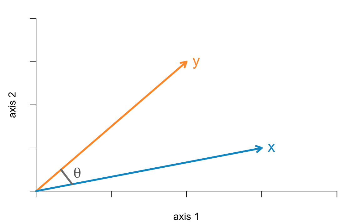
Figure 3.11: Two vectors in a 2-dimensional space
The inner product ot two mean-centered vectors \(\langle \mathbf{x}, \mathbf{y} \rangle\) is obtained with the following equation:
\[ \mathbf{x^{\mathsf{T}} y} = \|\mathbf{x}\| \hspace{1mm} \|\mathbf{y}\| \hspace{1mm} cos(\theta_{x,y}) \tag{3.43} \]
where \(cos(\theta_{x,y})\) is the angle between \(\mathbf{x}\) and \(\mathbf{y}\). Rearranging the terms in the previous equation we get that:
\[ cos(\theta_{x,y}) = \frac{\mathbf{x^\mathsf{T} y}}{\|\mathbf{x}\| \hspace{1mm} \|\mathbf{y}\|} = cor(\mathbf{x, y}) \tag{3.44} \]
which means that the correlation between mean-centered vectors \(\mathbf{x}\) and \(\mathbf{y}\) turns out to be the cosine of the angle between \(\mathbf{x}\) and \(\mathbf{y}\).
3.4.8 Orthogonal Projections
Last but not least, we finish this chapter with a discussion of projections. To be more specific, the statistical interpretation of orthogonal projections.
Let’s motivate this discussion with the following question: Consider two variables \(\mathbf{x}\) and \(\mathbf{y}\). Can we approximate one of the variables in terms of the other? This is an asymmetric type of association since we seek to say something about the variability of one variable, say \(\mathbf{y}\), in terms of the variability of \(\mathbf{x}\).

Figure 3.12: Two vectors in n-dimensional space
We can think of several ways to approximate \(\mathbf{y}\) in terms of \(\mathbf{x}\). The approximation of \(\mathbf{y}\), denoted by \(\mathbf{\hat{y}}\), means finding a scalar \(b\) such that:
\[ \mathbf{\hat{y}} = b \mathbf{x} \tag{3.45} \]
The common approach to get \(\mathbf{\hat{y}}\) in some optimal way is by minimizing the square difference between \(\mathbf{y}\) and \(\mathbf{\hat{y}}\).

Figure 3.13: Orthogonal projection of y onto x
The answer to this question comes in the form of a projection. More precisely, we orthogonally project \(\mathbf{y}\) onto \(\mathbf{x}\):
\[ \mathbf{\hat{y}} = \mathbf{x} \left( \frac{\mathbf{y^\mathsf{T} x}}{\mathbf{x^\mathsf{T} x}} \right) \tag{3.46} \]
or equivalently:
\[ \mathbf{\hat{y}} = \mathbf{x} \left( \frac{\mathbf{y^\mathsf{T} x}}{\| \mathbf{x} \|^2} \right) \tag{3.47} \]
For convenience purposes, we can rewrite the above equation in a slightly different format:
\[ \mathbf{\hat{y}} = \mathbf{x} (\mathbf{x^\mathsf{T}x})^{-1} \mathbf{x^\mathsf{T}y} \tag{3.48} \]
If you are familiar with linear regression, you should be able to recognize this equation. We’ll come back to this when we get to the chapter about Linear regression.
3.4.9 The mean as an orthogonal projection
Let’s go back to the concept of mean of a variable. As we previously mention, a variable \(X = (x_1, \dots, x_n)\), can be thought of a vector \(\mathbf{x}\) in an \(n\)-dimensional space. Furthermore, let’s also consider the constant vector \(\mathbf{1}\) of size \(n\). Here’s a conceptual diagram for this situation:

Figure 3.14: Two vectors in n-dimensional space
Out of curiosity, what happens when we ask about the orthogonal projection of \(\mathbf{x}\) onto \(\mathbf{1}\)? Something like in the following picture:

Figure 3.15: Orthogonal projection of vector x onto constant vector 1
This projection is expressed in vector notation as:
\[ \mathbf{\hat{x}} = \mathbf{1} \left( \frac{\mathbf{x^\mathsf{T} 1}}{\mathbf{1^\mathsf{T} 1}} \right) \tag{3.49} \]
or equivalently:
\[ \mathbf{\hat{x}} = \mathbf{1} \left( \frac{\mathbf{x^\mathsf{T} 1}}{\| \mathbf{1} \|^2} \right) \tag{3.50} \]
Note that the term in parenthesis is just a scalar, so we can actually express \(\mathbf{\hat{x}}\) as \(b \mathbf{1}\). This means that a projection implies multiplying \(\mathbf{1}\) by some number \(b\), such that \(\mathbf{\hat{x}} = b \mathbf{1}\) is a stretched or shrinked version of \(\mathbf{1}\). So, what is the scalar \(b\)? It is simply the mean of \(\mathbf{x}\):
\[ \mathbf{\hat{x}} = \mathbf{1} \left( \frac{\mathbf{x^\mathsf{T} 1}}{\| \mathbf{1} \|^2} \right) = \bar{x} \mathbf{1} \tag{3.51} \]
This is better appreciated in the following figure.

Figure 3.16: Mean of x and its relation with the projection onto constant vector 1
What this tells us is that the mean of the variable \(X\), denoted by \(\bar{x}\), has a very interesting geometric interpretation. As you can tell, \(\bar{x}\) is the scalar by which you would multiply \(\mathbf{1}\) in order to obtain the vector projection \(\mathbf{\hat{x}}\).