26 Preamble for Discriminant Analysis
We now turn our attention to a different kind of classification methods that belong to a general framework known as Dicriminant Analysis. In this chapter, we introduce some preliminary concepts that should allow you to have a better understanding of some underlying ideas behind discriminant analysis methods. The starting point involves discussing some aspects that are typically studied in Analysis of Variance (ANOVA). Overall, we focus on certain notions and formulas to measure variation (or dispersion) within classes and between classes. Now, keep in mind that we won’t describe any inferential aspects that are commonly used in statistical tests for comparing means of classes.
26.1 Motivation
Let’s consider the famous Iris data set collected by Edgar Anderson (1935), and used by Ronald Fisher (1936) in his seminal paper about Discriminant Analysis: The use of multiple measurements in taxonomic problems.
This data consists of 5 variables measured on \(n = 150\) iris flowers. There are \(p\) = 4 predictors, and one response. The four variables are:
Sepal.LengthSepal.WidthPetal.LengthPetal.Width
The response is a categorical (i.e. qualitative) variables that indicates the species of iris flower with three categories:
setosaversicolorvirginica
We should say that the iris data set is a classic textbook example. It is:
- clean data
- tidy data
- classess are fairly well separated
- size of data (small)
- good for learning and teaching purposes
Keep in mind that most real data sets won’t be like the iris data.
#>   Sepal.Length Sepal.Width Petal.Length Petal.Width Species
#> 1          5.1         3.5          1.4         0.2  setosa
#> 2          4.9         3.0          1.4         0.2  setosa
#> 3          4.7         3.2          1.3         0.2  setosa
#> 4          4.6         3.1          1.5         0.2  setosa
#> 5          5.0         3.6          1.4         0.2  setosa
#> 6          5.4         3.9          1.7         0.4  setosa
Some summary statistics:
#>   Sepal.Length    Sepal.Width     Petal.Length    Petal.Width
#>  Min.   :4.300   Min.   :2.000   Min.   :1.000   Min.   :0.100
#>  1st Qu.:5.100   1st Qu.:2.800   1st Qu.:1.600   1st Qu.:0.300
#>  Median :5.800   Median :3.000   Median :4.350   Median :1.300
#>  Mean   :5.843   Mean   :3.057   Mean   :3.758   Mean   :1.199
#>  3rd Qu.:6.400   3rd Qu.:3.300   3rd Qu.:5.100   3rd Qu.:1.800
#>  Max.   :7.900   Max.   :4.400   Max.   :6.900   Max.   :2.500
#>        Species
#>  setosa    :50
#>  versicolor:50
#>  virginica :50
#>
#>
#>
Let’s look at the distribution of the four input variables without making distinction between species of iris flowers:
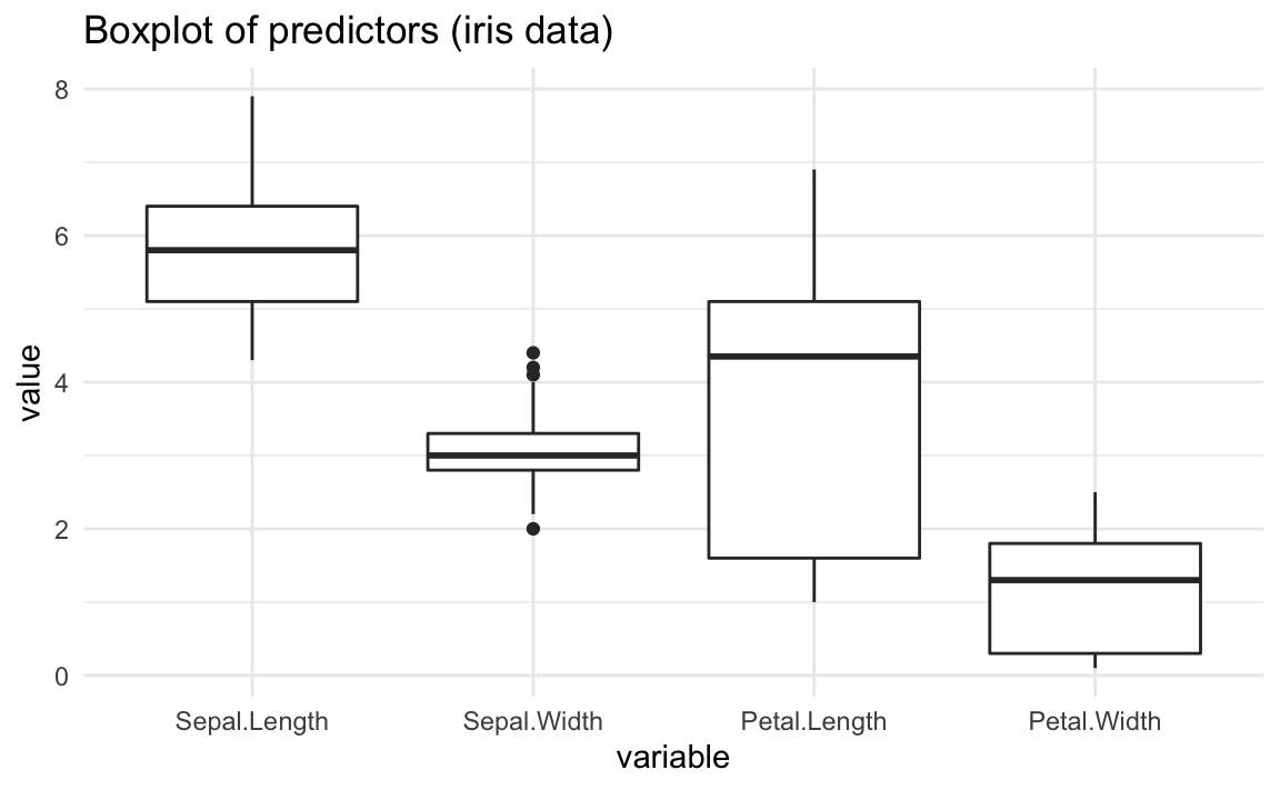
As you can tell from the above conditional boxplots, all predictors have different ranges, as well as different types of distributions.
Now let’s take into account the group structure according to the species:
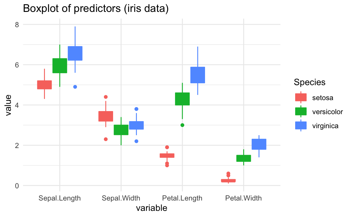
You should be able to observe that the boxplot of some predictors are fairly
different between iris species. For example, take a look at the boxplots of
Petal.Length, and the boxplots of Petal.Width. In contrast, predictors like
Sepal.Length and Sepal.Width have boxplots that are not as different as
those of Petal.Length.
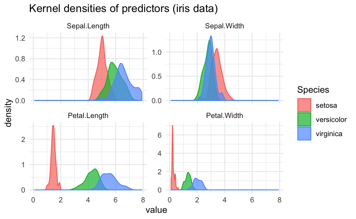
The same differences can be seen if we take a look at density curves:
26.1.1 Distinguishing Species
Let us consider the following question:
Which predictor provides the “best” distinction between Species?
- In classification problems, the response variable \(Y\) provides a group or class structure to the data.
- We expect that the predictors will help us to differentiate (i.e. discriminate) between one class and the others.
- The general idea is to look for systematic differences among classes. But how?
- A “natural” way to look for differences is paying attention to class means.
Let’s begin with a single predictor \(X\) and a categorical response \(Y\) measured on \(n\) individuals. Let’s take into account the class structure conveyed by \(Y\)
- Assume there are \(K\) classes (or categories)
- Let \(\mathcal{C_k}\) represent the \(k\)-th class in \(Y\)
- Let \(n_k\) be the number of observations in class \(\mathcal{C_k}\),
Then:
\[ n = n_1 + n_2 + \dots + n_K = \sum_{k=1}^{K} n_k \tag{26.1} \]
The (global) mean value of \(X\) is:
\[ \bar{x} = \frac{1}{n} \sum_{i=1}^{n} x_i \tag{26.2} \]
Each class \(k\) will have its mean \(\bar{x}_k\):
\[ \bar{x}_k = \frac{1}{n_k} \sum_{i \in \mathcal{C_k}} x_{ik} \tag{26.3} \]
#> overall mean of Sepal.Length
#> [1] 5.843333
Recall that a measure of (global) dispersion in \(X\) is given by the total sum of squares (\(\text{tss}\)):
\[ \text{tss} = \sum_{i=1}^{n} (x_i - \bar{x})^2 \tag{26.4} \]
#> total sums-of-squares of Sepal.Length
#> [1] 102.1683
Each class \(k\) will also have its own sum-of-squares \(\text{ss}_k\)
\[ \text{ss}_k = \sum_{i \in \mathcal{C_k}} (x_{ik} - \bar{x}_k)^2 \tag{26.5} \]
One way to look for systematic differences between the classes is to compare their means. If there’s no group difference in \(X\), then the group means \(\bar{x}_{k}\) should be similar. If there is really a difference, it is likely that one or more of the mean values will differ.
A useful measure to compare differences among the \(k\) means is the deviation from the overall mean:
\[ \bar{x}_{k} - \bar{x} \]
An effective summary of these deviations is the so-called between-group sum of squares (\(\text{bss}\)) given by:
\[ \text{bss} = \sum_{k=1}^{K} n_k (\bar{x}_{k} - \bar{x})^2 \tag{26.6} \]
#> between sums-of-squares of Sepal.Length
#> [1] 63.21213
To assess the relative magnitude of the between sum of squares (\(\text{bss}\)), we need to compare it to a measure of the “background” variation.
Such a measure of background variation can be formed by combining the group variances into a pooled-estimate called within-group sum of squares (\(\text{wss}\)):
\[ \text{wss} = \sum_{k=1}^{K} \sum_{i \in \mathcal{C_k}} (x_{ik} - \bar{x}_k)^2 = \text{ss}_1 + \dots + \text{ss}_K \tag{26.7} \]
#> within sums-of-squares of Sepal.Length
#> [1] 38.9562
So far we have three types of sums of squares:
\[\begin{align*} \textsf{total} \quad \text{tss} &= \sum_{i=1}^{n} (x_i - \bar{x})^2\\ \textsf{between} \quad \text{bss} &= \sum_{k=1}^{K} n_k (\bar{x}_{k} - \bar{x})^2 \\ \textsf{within} \quad \text{wss} &= \sum_{k=1}^{K} \sum_{i \in \mathcal{C_k}} (x_{ik} - \bar{x}_k)^2 \tag{26.8} \end{align*}\]
26.1.2 Sum of Squares Decomposition
An important aspect has to do with looking at the squared deviations, \((x_{i} - \bar{x})^2\), in terms of the class structure.
A useful trick is to rewrite the deviation terms \(x_{i} - \bar{x}\) as:
\[\begin{align*} x_{i} - \bar{x} &= x_{i} - (\bar{x}_{k} - \bar{x}_{k}) - \bar{x} \\ &= (x_{i} - \bar{x}_{k}) + (\bar{x}_{k} - \bar{x}) \tag{26.9} \end{align*}\]
We can decompose \(\text{tss}\) in terms of \(\text{bss}\) and \(\text{wss}\) as follows:
\[ \underbrace{\sum_{k=1}^{K} \sum_{i \in \mathcal{C_k}} (x_{ik} - \bar{x})^2}_{\text{tss}} = \underbrace{\sum_{k=1}^{K} n_k (\bar{x}_k - \bar{x})^2}_{\text{bss}} + \underbrace{\sum_{k=1}^{K} \sum_{i \in \mathcal{C_k}} (x_{ik} - \bar{x}_k)^2}_{\text{wss}} \tag{26.10} \]
In summary:
\[ \text{tss} = \text{bss} + \text{wss} \tag{26.11} \]
26.2 Derived Ratios from Sum-of-Squares
We now present two ratios derived from these sums of squares:
- Correlation ratio
- F-ratio
26.2.1 Correlation Ratio
The correlation ratio is a measure of the relationship between the dispersion within groups and the dispersion across all individuals.
Correlation ratio \(\eta^2\) (originally proposed by Karl Pearson) is given by:
\[ \eta^2(X,Y) = \frac{\text{bss}}{\text{tss}} \tag{26.12} \]
- \(\eta^2\) takes vaues between 0 and 1.
- \(\eta^2 = 0\) represents the special case of no dispersion among the means of the different groups.
- \(\eta^2 = 1\) refers to no dispersion within the respective groups.
#> correlation ratio of Sepal Length and Species
#> [1] 0.6187057
26.2.2 F-Ratio
With \(\text{tss} = \text{bss} + \text{wss}\), we can also calculate the \(F\)-ratio (proposed by R.A. Fisher):
\[ F = \frac{\text{bss} / (K-1)}{\text{wss} / (n-K)} \tag{26.13} \]
The larger the value of both ratios, the more variability is there between groups than within groups.
#> F-ratio of Sepal Length and Species
#> [1] 119.2645
The \(F\)-ratio can be used for hypothesis testing purposes. More formally, a null hypothesis postulates that the population means do not differ (\(H_0: \mu_1 = \mu_2 = \dots = \mu_K = \mu)\) versus the alternative hypothesis \(H_1\) that one or more population means differ among the \(K\) normally distributed populations.
Assuming or knowing that the variances of each sampled population are the same \(\sigma^2\), a test statistic to assess the null hypothesis is:
\[ F = \frac{\text{bss} / (K-1)}{\text{wss} / (n-K)} \tag{26.14} \]
which has an \(F\)-distribution with \(K-1\) and \(n-K\) degrees of freedom under the null hypothesis.
Example with Iris data
Let’s compute the dispersion decompositions for all predictors, and obtain the correlation ratios and \(F\)-ratios
#> correlation ratios
#> Sepal.Length  Sepal.Width Petal.Length  Petal.Width
#>    0.6187057    0.4007828    0.9413717    0.9288829
#> F-ratios
#> Sepal.Length Sepal.Width Petal.Length Petal.Width
#> 119.26450 49.16004 1180.16118 960.0071526.3 Geometric Perspective
As we’ve been doing throughout most chapters in the book, let’s provide a geometric perspective of what’s going on with the data, and the classification setting behind discriminant analysis. As usual, assume that the objects form a cloud of points in \(p\)-dimensional space.

Figure 26.1: Cloud of n points in p-dimensional space
One of the things that we can do is to look at the average individual, denoted by \(\mathbf{g}\), also known as the global centroid (i.e. the center of gravity of the cloud of points).

Figure 26.2: The centroid of the cloud of points
The global centroid \(\mathbf{g}\) is the point of averages which consists of the point formed with all the variable means:
\[ \mathbf{g} = [\bar{x}_1, \bar{x}_2, \dots, \bar{x}_p] \tag{26.15} \]
where:
\[ \bar{x}_j = \frac{1}{n} \sum_{i=1}^{n} x_{ij} \tag{26.16} \]
If all variables are mean-centered, the centroid is the origin
\[ \mathbf{g} = \underbrace{[0, 0, \dots, 0]}_{p \text{ times}} \tag{26.17} \]
Taking the global centroid as a point of reference, we can look at the amount of spread or dispersion in the data.
Assuming centered features, a matrix of total dispersion is given by the Total Sums of Squares (\(\text{TSS}\)):
\[ \text{TSS} = \mathbf{X^\mathsf{T} X} \tag{26.18} \]
Alternatively, we can get the (sample) variance-covariance matrix \(\mathbf{V}\):
\[ \mathbf{V} = \frac{1}{n-1} \mathbf{X^\mathsf{T} X} \tag{26.19} \]
26.3.1 Clouds from Class Structure
Here’s some notation that we’ll be using while covering some discriminant methods:
Let \(n_k\) be the number of observations in the \(k\)-th class
Let \(x_{ijk}\) represent the \(i\)-th observation, of the \(j\)-th variable, in the \(k\)-th class
Let \(x_{ik}\) represent \(i\)-th observation in class \(k\)
Let \(x_{jk}\) represent \(j\)-th variable in class \(k\)
Let \(n_k\) be the number of observations in the \(k\)-th class \(\mathcal{C_k}\)
The number of individuals: \(n = n_1 + n_2 + \dots + n_K = \sum_{k=1}^{K} n_k\)
Let’s now take into the account the class structure given by the response variable.

Figure 26.3: The objects are divided into classes or groups
Each class is denoted by \(\mathcal{C_k}\), and it is supposed to be formed by \(n_k\) individuals.

Figure 26.4: Each class forms its own sub-cloud
We can also look at the local or class centroids (one per class)

Figure 26.5: Each class has its own centroid
The class centroid \(\mathbf{g_k}\) is the point of averages for those observations in class \(k\):
\[ \mathbf{g_k} = [\bar{x}_{1k}, \bar{x}_{2k}, \dots, \bar{x}_{pk}] \tag{26.20} \]
where:
\[ \bar{x}_{jk} = \frac{1}{n_k} \sum_{i \in \mathcal{C_k}} x_{ij} \tag{26.21} \]
We can focus on the dispersion within the clouds

Figure 26.6: Dispersion within the sub-clouds
Each group will have an associated spread or dispersion matrix given by a Class Sums of Squares (\(\text{CSS}\)):
\[ \text{CSS}_k = \mathbf{X_{k}^{\mathsf{T}} X_k} \tag{26.22} \]
Equivalently, there is an associated variance matrix \(\mathbf{W_k}\) for each class
\[ \mathbf{W_k} = \frac{1}{n_k - 1} \mathbf{X_{k}^{\mathsf{T}} X_k} \tag{26.23} \]
where \(\mathbf{X_k}\) is the data matrix of the \(k\)-th class
We can combine the class dispersion to obtain a Within-class Sums of Squares (\(\text{WSS}\)) matrix:
\[\begin{align*} \text{WSS} &= \sum_{k=1}^{K} \mathbf{X_{k}^{\mathsf{T}} X_k} \\ &= \sum_{k=1}^{K} \text{CSS}_k \tag{26.24} \end{align*}\]
Likewise, we can combine the class variances \(\mathbf{W_k}\) as a weighted average to get the Within-class variance matrix \(\mathbf{W}\):
\[ \mathbf{W} = \sum_{k=1}^{K} \frac{n_k - 1}{n - 1} \mathbf{W_k} \tag{26.25} \]
What if we focus on just the centroids?

Figure 26.7: Global and Group Centroids
Note that the global centroid \(\mathbf{g}\) can be expressed as a weighted average of the group centroids:
\[\begin{align*} \mathbf{g} &= \frac{n_1}{n} \mathbf{g_1} + \frac{n_2}{n} \mathbf{g_2} + \dots + \frac{n_K}{n} \mathbf{g_K} \\ &= \sum_{k=1}^{K} \left ( \frac{n_k}{n} \right ) \mathbf{g_k} \tag{26.26} \end{align*}\]
Focusing on just the centroids, we can get its corresponding matrix of dispersion given by the Between Sums of Squares (\(\text{BSS}\)):
\[ \text{BSS} = \sum_{k=1}^{K} n_k (\mathbf{g_k - g})(\mathbf{g_k - g})^\mathsf{T} \tag{26.27} \]
Equivalently, there is an associated Between-class variance matrix \(\mathbf{B}\)
\[ \mathbf{B} = \sum_{k=1}^{K} \frac{n_k}{n - 1} (\mathbf{g_k - g})(\mathbf{g_k - g})^\mathsf{T} \tag{26.28} \]
Three types of Dispersions
Let’s recap. We have three types of sums-of-squares matrices:
- \(\text{TSS}\): Total Sums of Squares
- \(\text{WSS}\): Within-class Sums of Squares
- \(\text{BSS}\): Between-class Sums of Squares
Alternatively, we also have three types of variance matrices:
- \(\mathbf{V}\): Total variance
- \(\mathbf{W}\): Within-class variance
- \(\mathbf{B}\): Between-class variance
26.3.2 Dispersion Decomposition
It can be shown (Huygens theorem) for both, sums-of-squares and variances, that the total dispersion (TSS or \(\mathbf{V}\)) can be decomposed as:
\(\text{TSS} = \text{BSS} + \text{WSS}\)
\(\mathbf{V} = \mathbf{B} + \mathbf{W}\)
Let \(\mathbf{X}\) be the \(n \times p\) mean-centered matrix of predictors, and \(\mathbf{Y}\) be the \(n \times K\) dummy matrix of classes:
\(\text{TSS} = \mathbf{X^\mathsf{T} X}\)
\(\text{BSS} = \mathbf{X^\mathsf{T} Y (Y^\mathsf{T} Y)^{-1} Y^\mathsf{T} X}\)
\(\text{WSS} = \mathbf{X^\mathsf{T} (I - Y (Y^\mathsf{T} Y)^{-1} Y^\mathsf{T}) X}\)

Figure 26.8: Dispersion Decomposition