13 Resampling Approaches
In this chapter we discuss how to make the most of a limitted data set. We describe several resampling techniques to generate multiple training sets, as well as multiple evaluation sets that we can use for both the training phase and the pre-selection phase.
13.1 General Sampling Blueprint
The idea behind most common (re)sampling approaches is to have a way to generate multiple sets from just one data set. In statistical learning, the training set is the one on which we usually apply resampling methods.
Suppose we are interested in fitting a \(k\)-Nearest-Neighbor (\(k\)-NN) model. In particular, we want to fit a \(k\)-NN model with \(k=3\) neighbors. So let’s denote this type of model as \(\mathcal{H}_1\) hypothesis. The starting point is the training set \(\mathcal{D}_{train}\). Using a sampling mechanism we split the training set into two subsets. One of the subsets, that we denote as \(\mathcal{D}_{train-b}\), is used to train a model, denoted \(h_{1,b}\). The other subset, denoted \(\mathcal{D}_{eval-b}\), is used to evaluate \(h_{1,b}\) by calculating a validation error \(E_{eval-b}\).
The way the evaluation set is formed, is by taking those data points in \(\mathcal{D}_{train}\), that are not included in \(\mathcal{D}_{train-b}\), that is:
\[ \mathcal{D}_{eval-b} = \mathcal{D}_{train} \setminus \mathcal{D}_{train-b} \tag{13.1} \]
This procedure is repeated \(B\) times. At the end, we average all the evaluation errors to get a single measure indicating the typical performance for the particular type of trained models:
\[ E_{eval} = \frac{1}{B} \sum_{b=1}^{B} E_{eval-b} \tag{13.2} \]
In this hypothetical example, this average measure \(E_{eval}\) would be the typical performance of 3-NN models.
The figure below depicts the general (re)sampling regime:

Figure 13.1: General scheme for sampling approaches
What distinguishes each sampling approach is the size and way in which the random samples are generated to obtain the sets \(\mathcal{D}_{train-b}\). Two main sampling mechanisms are typically used: 1) random samples without replacement, or 2) random samples with replacement.
13.2 Monte Carlo Cross Validation
The first sampling method that we discuss is Monte-Carlo Cross-Validation, sometimes known as Repeated Holdout Method.
As the name indicates, this method repeatedly produces a holdout set, \(\mathcal{D}_{eval-b}\), to be used for evaluating the performance of a model. At each iteration (or repetition) \(b\) we split \(\mathcal{D}_{train}\) into \(\mathcal{D}_{train-b}\) and \(\mathcal{D}_{eval-b}\). We use the training subset \(\mathcal{D}_{train-b}\) to fit a particular model \(h^{-}_{b}\), and then we use the validation subset \(\mathcal{D}_{eval-b}\) to obtain \(E_{eval-b}\).

Figure 13.2: Several splits into training and evaluation sets
After several repetitions, we average all the test errors \(E_{eval-b}\) to obtain \(E_{eval}(h^{-})\), an estimate of \(E_{out}(h^{-})\).
Repeated Holdout Algorithm
Here’s the conceptual algorithm for the repeated holdout method:
Compile the training data into a set \(\mathcal{D}_{train} = \{(\mathbf{x_1}, y_1), \dots, (\mathbf{x_n}, y_n) \}\).
Repeat the Holdout method \(B\) times, where \(B\) is a very large integer (for example, 500). At each iteration, obtain the following elements:
Generate \(\mathcal{D}_{train-b}\), by sampling \(n-r\) elements without replacement from \(\mathcal{D}_{train}\).
Generate \(h^{-}_{b}\), by fitting a model to \(\mathcal{D}_{train-b}\)
Compute \(E_{eval-b} = \frac{1}{r} \sum_{i} err_i \big( h^{-}_{b}(\mathbf{x_i}), y_i \big)\); where \((\mathbf{x_i}, y_i) \in \mathcal{D}_{eval-b}\)
Obtain an overall value for \(E_{eval}\) by averaging the \(E_{eval-b}\) values:
\[ E_{eval} = \frac{1}{B} \sum_{b=1}^{B} E_{eval-b} \tag{13.3} \]
13.3 Bootstrap Method
Another interesting validation procedure is the “Bootstrap Method”.
This method is very similar to the Repeated Holdout method. The main difference is in the way \(\mathcal{D}_{train}\) is split in each repetition. In the bootstrap method, as the name says, the samples consists of bootstrap samples.
Recall that a bootstrap sample is a random sample of the data taken with replacement. This means that the bootstrap sample is the same size as elements in \(\mathcal{D}_{train}\). As a result, some individuals will be represented multiple times in the bootstrap sample while others will not be selected at all. The individuals not selected are usually referred to as the out-of-bag elements.

Figure 13.3: Several splits with bootstrap samples into training and test sets
Bootstrap Algorithm
Here’s the conceptual algorithm for the bootstrap method:
Compile the training data into a set \(\mathcal{D}_{train} = \{(\mathbf{x_1}, y_1), \dots, (\mathbf{x_n}, y_n) \}\).
Repeat the following steps for \(b = 1, 2, \dots B\) where \(B\) is a very large integer (for example, 500):
Generate \(\mathcal{D}_{train-b}\) by sampling \(n\) times with replacement from \(\mathcal{D}_{train}\). (Note that \(\mathcal{D}_{train-b}\) could contain repeated elements).
Generate \(\mathcal{D}_{eval-b}\) by combining all of the elements in \(\mathcal{D}_{train}\) that were not captured in \(\mathcal{D}_{train-b}\). Hence, the size of \(\mathcal{D}_{eval-b}\) will change at each iteration. (Note that \(\mathcal{D}_{eval-b}\) should not contain repeated values).
Generate \(h^{-}_b\) by fitting a model to \(\mathcal{D}_{train-b}\).
Compute \(E_{eval-b} = \frac{1}{r_b} \sum_{i} err_i \big( h^{-}_b(\mathbf{x_i}), y_i \big)\), where \((\mathbf{x_i}, y_i) \in \mathcal{D}_{eval-b}\) and \(r_b\) is the size of \(\mathcal{D}_{eval-b}\).
Obtain an overall value for bootstrap \(E_{eval}\) by averaging the \(E_{eval-b}\) values:
\[ \text{bootstrap } E_{eval} = \frac{1}{B} \sum_{b=1}^{B} E_{eval-b} \tag{13.4} \]
Bootstrapping enables us to construct confidence intervals for \(E_{out}\). We have that:
\[ \mathrm{SE}_{boot} = \sqrt{ \frac{1}{B - 1} \sum_{b=1}^{B} \left(E_{eval-b} - E_{eval} \right)^2 } \tag{13.5} \]
Empirical quantiles can be used.
13.4 \(K\)-Fold Cross-Validation
The idea of the classic cross-validation method (not to confuse with monte carlo cross-validation) is to split the training data into \(K\) sets of equal (or almost equal) size. Each of the resulting subsets is referred to as a fold. Usually, the way in which the folds are formed is by randomly splitting the initial data.
The diagram below illustrates a 3-fold cross validation sampling scheme:

Figure 13.4: 3-fold splits
As you can tell, the training data is (randomly) divided into three sets of similar size: the 3-folds. Then, at each iteration \(b\), one of the folds is held out for evaluation purposes, i.e. \(\mathcal{D}_{eval-b}\); the reamining folds are merged into \(\mathcal{D}_{train-b}\), and used for training purposes. As usual, at the end of the iterations (\(b = K\)), all evaluation errors \(E_{eval-b}\) are aggregated into an average \(E_{eval}\), commonly known as the cross-validation error \(E_{cv}\).
13.4.1 Leave-One-Out Cross Validation (LOOCV)
One special case of \(K\)-fold cross-validation is when each fold consists of a single data point, that is \(K = n\). This particular scheme is known as leave-one-out cross-validation (loocv). Let’s see how to carry out loocv.
Compile the training data into a set \(\mathcal{D}_{train} = \{(\mathbf{x_1}, y_1), \dots, (\mathbf{x_n}, y_n) \}\).
Repeat the following for \(i = 1, 2, \dots, n\) (where \(n\) is the number of data points)
Generate the \(i\)-th training set \(\mathcal{D}_i\) by removing the \(i\)-th element from \(\mathcal{D}_{train}\); that is, \(\mathcal{D}_i = \mathcal{D} \backslash \{ (\mathbf{x_i}, y_i) \}\).
Fit your model to \(\mathcal{D}_i\) to obtain model \(h_{i}^{-}\)
Use the point \((\mathbf{x_i}, y_i)\) that is left-out to compute \(E_{eval-i} = err \big( h_{i}^{-}(\mathbf{x_i}), y_i \big)\).
Obtain the cross-validation error \(E_{cv}\) by averaging the individual errors:
\[ E_{cv} = \frac{1}{n} \sum_{i=1}^{n} err_i = \frac{1}{n} \sum_{i=1}^{n} E_{eval-i} \tag{13.6} \]
In this way, we are able to fit \(n\) models with \(n - 1\) points, while also generating \(n\) testing datasets. So, this looks like the best of both worlds: we have a large training data set, and a lot of test datasets! But, there is still a cost: the individual errors are no longer independent.
For illustrative purposes, consider a data set withonly three points: \(\mathcal{D} = \{p_1, p_2, p_3\}\) (pictured below).
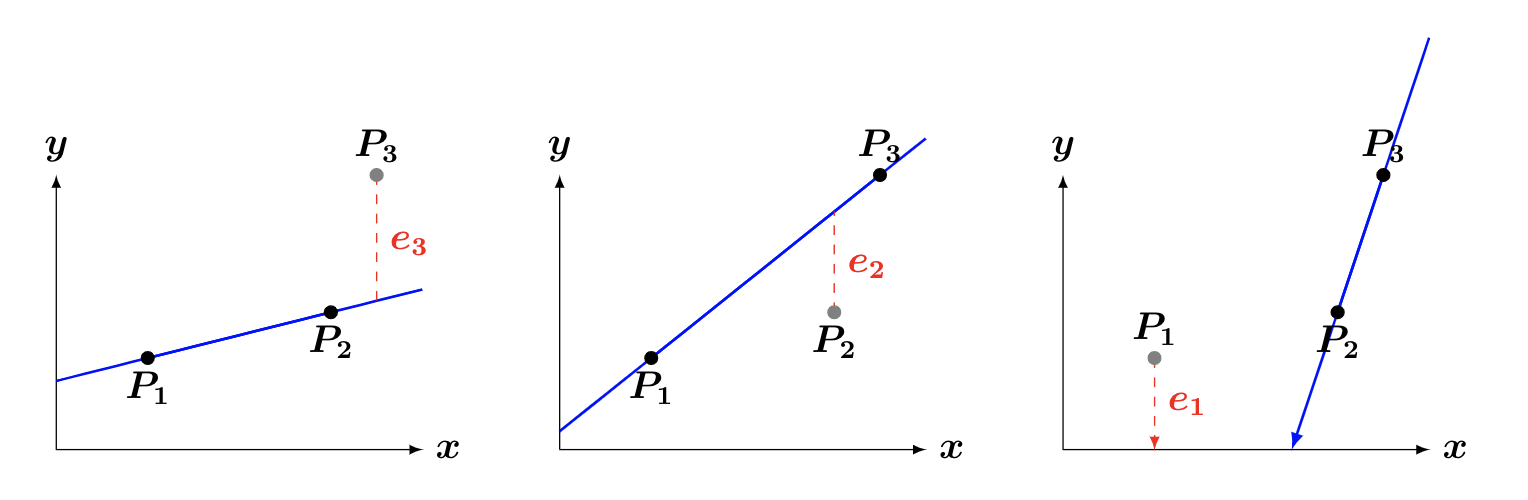
Figure 13.5: Illustration of loocv errors
We would therefore repeat step (2) above \(n = 3\) times, to obtain \(3\) errors: \(e_1, \ e_2,\) and \(e_3\) [note that in the last figure, the red dashed line extends to touch the blue line; unfortunately, the point of intersection was too low to feasibly show on the graph. In other words, use your imagination: the red line touches the blue line].