16 Partial Least Squares Regression
Another dimension reduction method that we can use to regularize a model is Partial Least Squares Regression (PLSR).
Before we dive deep into the nuts and bolts of PLSR, we should let you know that PLS methods form a very big family of methods. While the regression method is probably the most popular PLS technique, it is by no means the only one. And even within PLSR, there’s a wide array of different algorithms that let you obtain the core solution.
PLS Regression was mainly developed in the early 1980s by Scandinavian chemometricians Svante Wold and Harald Martens. The theoretical background was based on the PLS Modeling framework of Herman Wold (Svante’s father).
- PLS Regression was developed as an algorithmic solution, with no optimization criterion explicitly defined.
- It was introduced in the fields of chemometrics (where almost immediately became a hit).
- It slowly attracted the attention of curious applied statisticians.
- It took a couple of years (late 1980s - early 1990s) for applied mathematicians to discover its properties.
- Nowadays there are several versions (flavors) of the algorithm to compute a PLS regression.
16.1 Motivation Example
To introduce PLSR we are using the same data set of the previous chapter: a subset of the “2004 New Car and Truck Data”. The data set consists of 10 variables measured on 385 cars. Here’s what the first six rows look like:
                              price engine cyl  hp city_mpg
Acura 3.5 RL 4dr              43755    3.5   6 225       18
Acura 3.5 RL w/Navigation 4dr 46100    3.5   6 225       18
Acura MDX                     36945    3.5   6 265       17
Acura NSX coupe 2dr manual S  89765    3.2   6 290       17
Acura RSX Type S 2dr          23820    2.0   4 200       24
Acura TL 4dr                  33195    3.2   6 270       20
                              hwy_mpg weight wheel length width
Acura 3.5 RL 4dr                   24   3880   115    197    72
Acura 3.5 RL w/Navigation 4dr      24   3893   115    197    72
Acura MDX                          23   4451   106    189    77
Acura NSX coupe 2dr manual S       24   3153   100    174    71
Acura RSX Type S 2dr               31   2778   101    172    68
Acura TL 4dr                       28   3575   108    186    72
The response variable is price, and there are nine predictors:
engine: engine size (liters)cyl: number of cylindershp: horsepowercity_mpg: city miles per gallonhw_mpg: highway miles per gallonweight: weights (pounds)wheel: wheel base (inches)length: length (inches)width: width (inches)
The regression model involves predicting price in terms of the nine inputs:
\[ \texttt{price} = b_0 + b_1 \texttt{cyl} + b_2 \texttt{hp} + \dots + b_9 \texttt{width} + \boldsymbol{\varepsilon} \tag{16.1} \]
Computing the OLS solution for the regression model of price onto the
other nine predictors we obtain the following coefficients (see first column):
              Estimate  Std. Error  t value   Pr(>|t|)
(Intercept)  32536.025   17777.488   1.8302  6.802e-02
engine       -3273.053    1542.595  -2.1218  3.451e-02
cyl           2520.927     896.202   2.8129  5.168e-03
hp             246.595      13.201  18.6797  1.621e-55
city_mpg      -229.987     332.824  -0.6910  4.900e-01
hwy_mpg        979.967     345.558   2.8359  4.817e-03
weight           9.937       2.045   4.8584  1.741e-06
wheel         -695.392     172.896  -4.0220  6.980e-05
length          33.690      89.660   0.3758  7.073e-01
width         -635.382     306.344  -2.0741  3.875e-02
16.2 The PLSR Model
In PLS regression, like in PCR, we seek components \(\mathbf{z_1}, \dots, \mathbf{z_k}\), linear combinations of the inputs (e.g. \(\mathbf{z_1} = \mathbf{Xw_1}\)). Unlike PCR, in PLS we want to obtain components such that they are good predictors for both the response \(\mathbf{y}\) as well as the inputs \(\mathbf{x_j}\) for \(j = 1,\dots, p\).
Moreover, there is an implicit assumption in the PLS regression model: both \(\mathbf{X}\) and \(\mathbf{y}\) are assumed to be functions of a reduced (\(k < p\)) number of components \(\mathbf{Z} = [\mathbf{z_1}, \dots, \mathbf{z_k}]\) that can be used to decompose the inputs and the response as follows:
\[ \mathbf{X} = \mathbf{Z V^\mathsf{T}} + \mathbf{E} \tag{16.2} \]

Figure 16.1: Matrix diagram for inputs
and
\[ \mathbf{y} = \mathbf{Z b} + \mathbf{e} \tag{16.3} \]

Figure 16.2: Matrix diagram for response
where:
- \(\mathbf{Z}\) is a matrix of PLS components
- \(\mathbf{V}\) is a matrix of PLS loadings
- \(\mathbf{E}\) is a matrix of \(X\)-residuals
- \(\mathbf{b}\) is a vector of PLS regression coefficients
- \(\mathbf{e}\) is a vector of \(y\)-residuals
By taking a few number of components \(\mathbf{Z} = [\mathbf{z_1}, \dots, \mathbf{z_k}]\), we can have approximations for the inputs and the response. The model for the \(X\)-space is:
\[ \mathbf{\hat{X}} = \mathbf{Z V^{\mathsf{T}}} \tag{16.4} \]
In turn, the prediction model for \(\mathbf{y}\) is given by:
\[ \mathbf{\hat{y}} = \mathbf{Z b} \tag{16.5} \]
To avoid confusing the PLSR coefficients with the OLS coefficients, or the PCR coefficients, we can be more proper and rewrite the previous expression as:
\[ \mathbf{\hat{y}} = \mathbf{Z} \mathbf{b}^{\text{pls}} \tag{16.6} \]
to indicate that the obtained \(b\)-coefficients are those associated to the PLS components.
16.3 How does PLSR work?
So how do we obtain the PLS components, aka PLS scores? We use an iterative algorithm, obtaining one component at a time. Here’s how to get the first PLS component \(\mathbf{z_1}\).
Assume that both the inputs and the response are mean-centered (and possibly standardized). We compute the covariances between all the input variables and the response: \(\mathbf{\tilde{w}_1} = (cov(\mathbf{x_1}, \mathbf{y}), \dots, cov(\mathbf{x_p}, \mathbf{y}))\).

Figure 16.3: Towards the first PLS component.
In vector-matrix notation we have:
\[ \mathbf{\tilde{w}_1} = \mathbf{X^\mathsf{T}y} \tag{16.7} \]
Alternatively, we can also obtain a rescaled version of \(\mathbf{\tilde{w}_1}\) by regressing each predictor \(\mathbf{x_j}\) onto \(\mathbf{y}\). Notice that this alternative option won’t change the direction of the covariances \(cov(\mathbf{x_j}, \mathbf{y})\). In vector-matrix notation we have:
\[ \mathbf{\tilde{w}_1} = \mathbf{X^\mathsf{T}y} / \mathbf{y^\mathsf{T} y} \tag{16.8} \]
For convenience purposes, we normalize the vector of covariances \(\mathbf{\tilde{w}_1}\), in order to get a unit-vector \(\mathbf{w_1}\):
\[ \mathbf{w_1} = \frac{\mathbf{\tilde{w}_1}}{\|\mathbf{\tilde{w}_1}\|} \tag{16.9} \]
first PLS weight
                 [,1]
engine    0.001782118
cyl       0.002857956
hp        0.171985612
city_mpg -0.007484109
hwy_mpg  -0.007752089
weight    0.984987298
wheel     0.004225081
length    0.008131684
width     0.003089621
We use these weights to compute the first component \(\mathbf{z_1}\) as a linear combination of the inputs:
\[ \mathbf{z_1} = w_{11} \mathbf{x_1} + \dots + w_{p1} \mathbf{x_p} \tag{16.10} \]

Figure 16.4: First PLS component.
Because \(\mathbf{w_1}\) is unit-vector, the formula for \(\mathbf{z_1}\) can be expressed like:
\[ \mathbf{z_1} = \mathbf{Xw_1} = \mathbf{Xw_1} / \mathbf{w_1^\mathsf{T} w_1} \tag{16.11} \]
Here are the first 10 elements of \(\mathbf{z_1}\)
first PLS component (10 elements only)
                                    [,1]
Acura 3.5 RL 4dr               344.24572
Acura 3.5 RL w/Navigation 4dr  357.05055
Acura MDX                      913.48050
Acura NSX coupe 2dr manual S  -360.90753
Acura RSX Type S 2dr          -745.89228
Acura TL 4dr                    51.39841
Acura TSX 4dr                 -300.53740
Audi A4 1.8T 4dr              -284.07748
Audi A4 3.0 4dr                -68.58479
Audi A4 3.0 convertible 2dr    278.15085
We use this component to regress both the inputs and the response onto it. The regression coefficient \(v_{1j}\) of each simple linear regression between \(\mathbf{z_1}\) and the \(j\)-th predictor is called a PLS loading. The entire vector of loadings \(\mathbf{v_1}\) associated to first component is:
\[ \mathbf{v_1} = \mathbf{X^\mathsf{T}z_1} / \mathbf{z_{1}^\mathsf{T}z_1} \tag{16.12} \]
first PLS loading
                 [,1]
engine    0.001176718
cyl       0.001561745
hp        0.064016991
city_mpg -0.005536001
hwy_mpg  -0.006343509
weight    1.003819205
wheel     0.007551534
length    0.012276141
width     0.003862309
In turn, the PLS regression coefficient \(b_1\) is obtained by regressing the response onto the first component:
\[ b_1 = \mathbf{y^\mathsf{T} z_1} / \mathbf{z_{1}^\mathsf{T}z_1} \tag{16.13} \]
In our example, the regression coefficient \(b_1\) of the first PLS score \(\mathbf{z_1}\) is:
first PLS regression coefficient
[1] 13.61137
We can then get a first one-rank approximation \(\mathbf{\hat{X}} = \mathbf{z_1 v^{\mathsf{T}}_1}\), and then obtain a residual matrix \(\mathbf{X_1}\) by removing the variation in the inputs captured by \(\mathbf{z_1}\) (this operation is known as deflation):
\[ \mathbf{X_1} = \mathbf{X} - \mathbf{\hat{X}} = \mathbf{X} - \mathbf{z_1 v^{\mathsf{T}}_1} \qquad \mathsf{(deflation)} \tag{16.14} \]
We can also deflate the response:
\[ \mathbf{y_1} = \mathbf{y} - b_1 \mathbf{z_1} \tag{16.15} \]
We can obtain further PLS components \(\mathbf{z_2}\), \(\mathbf{z_3}\), etc. by repeating the process described above on the residual data matrices \(\mathbf{X_1}\), \(\mathbf{X_2}\), etc., and the residual response vectors \(\mathbf{y_1}\), \(\mathbf{y_2}\), etc. For example, a second PLS score \(\mathbf{z_2}\) will be formed by a linear combination of first \(X\)-residuals:

Figure 16.5: Second PLS component.
16.4 PLSR Algorithm
We will describe what we consider the “standard” or “classic” algorithm. However, keep in mind that there are a handful of slightly different versions that you may find in other places.
We assume mean-centered and standardized variables \(\mathbf{X}\) and \(\mathbf{y}\).
- We start by setting \(\mathbf{X_0} = \mathbf{X}\), and \(\mathbf{y_0} = \mathbf{y}\).
Repeat for \(h = 1, \dots, r = \text{rank}(\mathbf{X})\):
Start with weights \(\mathbf{\tilde{w}_h} = \mathbf{X_{h-1}^\mathsf{T}} \mathbf{y_{h-1}} / \mathbf{y_{h-1}}^\mathsf{T} \mathbf{y_{h-1}}\)
Normalize weights: \(\mathbf{w_h} = \mathbf{\tilde{w}_h} / \| \mathbf{\tilde{w}_h} \|\)
Compute PLS component: \(\mathbf{z_h} = \mathbf{X_{h-1} w_h} / \mathbf{w_{h}^\mathsf{T} w_h}\)
Regress \(\mathbf{y_h}\) onto \(\mathbf{z_h}\): \(b_h = \mathbf{y_{h}^{\mathsf{T}} z_h / z_{h}^{\mathsf{T}} z_h}\)
Regress all \(\mathbf{x_j}\) onto \(\mathbf{z_h}\): \(\mathbf{v_h} = \mathbf{X_{h-1}}^{\mathsf{T}} \mathbf{z_h} / \mathbf{z_{h}}^{\mathsf{T}} \mathbf{z_h}\)
Deflate (residual) predictors: \(\mathbf{X_h} = \mathbf{X_{h-1}} - \mathbf{z_h} \mathbf{v_{h}^{\mathsf{T}}}\)
Deflate (residual) response: \(\mathbf{y_h} = \mathbf{y_{h-1}} - b_h \mathbf{z_h}\)
Notice that steps 1, 3, 4, and 5 involve simple OLS regressions. If you think about it, what PLS is doing is calculating all the different ingredients (e.g. \(\mathbf{w_h}, \mathbf{z_h}, \mathbf{v_h}, b_h\)) separately, using least squares regressions. Hence the reason for its name partial least squares.
16.4.1 PLS Solution with original variables
More often than not, the PLS regression equation is typically expressed in terms of the original variables \(\mathbf{X}\) instead of using the PLS components \(\mathbf{Z}\). This re-arrangement is more convenient for interpretation purposes and makes it easy to work with the input features.
\[ \mathbf{\hat{y}} = \mathbf{Z b} \ \longrightarrow \ \mathbf{\hat{y}} = \mathbf{X \overset{*}{b}} \tag{16.16} \]
Note that the PLS \(X\)-coefficients \(\mathbf{\overset{*}{b}}\) are not parameters of the PLS regression model. Instead, these are post-hoc calculations for making things more maneagable. Let’s find out how to obtain these coefficients.
Transforming Regression Coefficients
Recall that PLS components are obtained as linear combinations of residual matrices \(\mathbf{X_h}\). Interestingly, PLS components can also be expressed in terms of the original variables.
The first component is directly expressed in terms of the input matrix \(\mathbf{X}\):
\[ \mathbf{z_1} = \mathbf{X w_1 = X \overset{*}{w}_{1}} \tag{16.17} \]
The second component is obtained in terms of the first residual matrix \(\mathbf{X_1}\), but we can reexpress it in terms of \(\mathbf{X}\):
\[\begin{align*} \mathbf{z_2} &= \mathbf{X_1 w_2} \\ &= (\mathbf{X} - \mathbf{z_1 v_{1}^\mathsf{T}}) \mathbf{w_2} \\ &= (\mathbf{X} - (\mathbf{Xw_1}) \mathbf{v_{1}^\mathsf{T}}) \mathbf{w_2} \\ &= \mathbf{X} \underbrace{(\mathbf{I} - \mathbf{w_1 v_{1}^\mathsf{T}}) \mathbf{w_2}}_{\mathbf{\overset{*}{w}_{2}}} \\ &= \mathbf{X \overset{*}{w}_{2}} \tag{16.18} \end{align*}\]
The third component is obtained in terms of the second residual matrix \(\mathbf{X_2}\), but we can also reexpress it in terms of \(\mathbf{X}\):
\[\begin{align*} \mathbf{z_3} &= \mathbf{X_2 w_3} \\ &= (\mathbf{X_1} - \mathbf{z_2 v_{2}^\mathsf{T}}) \mathbf{w_3} \\ &= (\mathbf{X_1} - \mathbf{X_1} \mathbf{w_2 v_{2}^\mathsf{T}}) \mathbf{w_3} \\ &= \mathbf{X_1} (\mathbf{I} - \mathbf{w_2 v_{2}^\mathsf{T}}) \mathbf{w_3} \\ &= \mathbf{X} \underbrace{(\mathbf{I} - \mathbf{w_1 v_{1}^\mathsf{T}}) (\mathbf{I} - \mathbf{w_2 v_{2}^\mathsf{T}}) \mathbf{w_3}}_{\mathbf{\overset{*}{w}_{3}}} \\ &= \mathbf{X \overset{*}{w}_{3}} \tag{16.19} \end{align*}\]
Consequently, \(\mathbf{Z_h} = [\mathbf{z_1}, \mathbf{z_2}, \dots, \mathbf{z_h}] = \mathbf{X \overset{*}{W}_{h}}\)
It can be proved that the matrix of star-vectors \(\mathbf{\overset{*}{W}_{h}} = [\mathbf{\overset{*}{w}_{1}}, \dots, \mathbf{\overset{*}{w}_{h}}]\) can be obtained with the following formula:
\[ \mathbf{\overset{*}{W}_{h}} = \prod_{k=1}^{h-1} (\mathbf{I} - \mathbf{w_k v_{k}^\mathsf{T}}) \mathbf{w_h} = \mathbf{W_h} (\mathbf{V_h^\mathsf{T} W_h})^{-1} \tag{16.20} \]
In summary, the PLS regression equation \(\mathbf{\hat{y}} = b_1 \mathbf{z_1} + \dots + b_h \mathbf{z_h} = \mathbf{Z b}\) can be expressed in terms of the original predictors as:
\[ \mathbf{\hat{y}} = \mathbf{Z b} = \mathbf{X \overset{*}{W} b} = \mathbf{X \overset{*}{b}} \tag{16.21} \]
where \(\overset{*}{\mathbf{b}}\) are the derived PLS \(X\)-coefficients (not OLS). Note that these PLS star-coefficients of the regression equation are NOT parameters of the PLS regression model. Instead, these are post-hoc calculations for making things more maneagable.

Figure 16.6: PLS components in terms of original inputs.
Interestingly, if you retain all \(h = rank(\mathbf{X})\) PLS components, the \(\overset{*}{\mathbf{b}}_\text{pls}\) coefficients will be equal to the OLS coefficients.
16.4.2 Some Properties
Some interesting properties of the different elements derived in PLS Regression:
\(\mathbf{z_h^{\mathsf{T}} z_l} = 0, \quad l > h\)
\(\mathbf{w_h^{\mathsf{T}} v_h} = 1\)
\(\mathbf{w_h^{\mathsf{T}} X_{l}^{\mathsf{T}}} = 0, \quad l \geq h\)
\(\mathbf{w_h^{\mathsf{T}} v_l} = 0, \quad l > h\)
\(\mathbf{w_h^{\mathsf{T}} w_l} = 0, \quad l > h\)
\(\mathbf{z_h^{\mathsf{T}} X_l} = 0, \quad l \geq h\)
\(\mathbf{X_h} = \mathbf{X} \prod_{j=1}^{p} (\mathbf{I - w_j v_{j}^{\mathsf{T}}}), \quad h \geq 1\)
16.4.3 PLS Regression for Price of cars
By default, we can obtain up to \(r = rank(\mathbf{X})\) different PLS components. In the cars example, we can actually obtain nine scores. The following output shows the regression coefficients—in terms of the input features—of all nine regression equations:
           Z_1:1  Z_1:2   Z_1:3   Z_1:4   Z_1:5   Z_1:6   Z_1:7    Z_1:8
engine    0.0243   1.44   -3.34  -15.09  -33.59 -113.70 -284.84 -1148.41
cyl       0.0389   3.03    6.87   55.93  166.51  471.47 1056.23  2073.22
hp        2.3410 250.04  248.74  262.63  254.81  251.35  243.73   238.81
city_mpg -0.1019  -4.69   50.66  368.94  210.79  -69.52 -412.43  -171.42
hwy_mpg  -0.1055  -3.49   48.59  464.50  528.56  811.07 1177.28   933.19
weight   13.4070  -2.27    1.80    6.44    8.21    9.61    9.77     9.08
wheel     0.0575  -7.32 -125.75 -387.68 -797.42 -669.88 -680.47  -676.98
length    0.1107  -9.00 -196.71  -90.85   83.57   59.30    2.26    17.07
width     0.0421  -1.61  -43.73 -181.27 -427.09 -940.70 -729.49  -725.37
            Z_1:9
engine   -3273.05
cyl       2520.93
hp         246.59
city_mpg  -229.99
hwy_mpg    979.97
weight       9.94
wheel     -695.39
length      33.69
width     -635.38
If we keep all components, we get the OLS solution (using standardized data):
Regression coefficients using all 9 PLS components
     engine         cyl          hp    city_mpg     hwy_mpg      weight
-3273.05304  2520.92691   246.59496  -229.98735   979.96656     9.93652
      wheel      length       width
 -695.39157    33.69009  -635.38224
Compare with the regression coefficients of OLS:
(Intercept)      engine         cyl          hp    city_mpg     hwy_mpg
32536.02465 -3273.05304  2520.92691   246.59496  -229.98735   979.96656
     weight       wheel      length       width
    9.93652  -695.39157    33.69009  -635.38224
Obviously, reatining all PLS scores does not provide an improvement over the OLS regression. This is because we are not changing anything. Using our metaphor about “shopping for coefficients”, by keeping all PLS scores we are spending the same amount of money that we spend in ordinary least-squares regression.
The dimension reduction idea involves keeping only a few components \(k \ll r\), such that the fitted model has a better generalization ability than the full model. The number of components \(k\) is called the tuning parameter or hyperparameter. How do we determine \(k\)? The typical way is to use cross-validation.
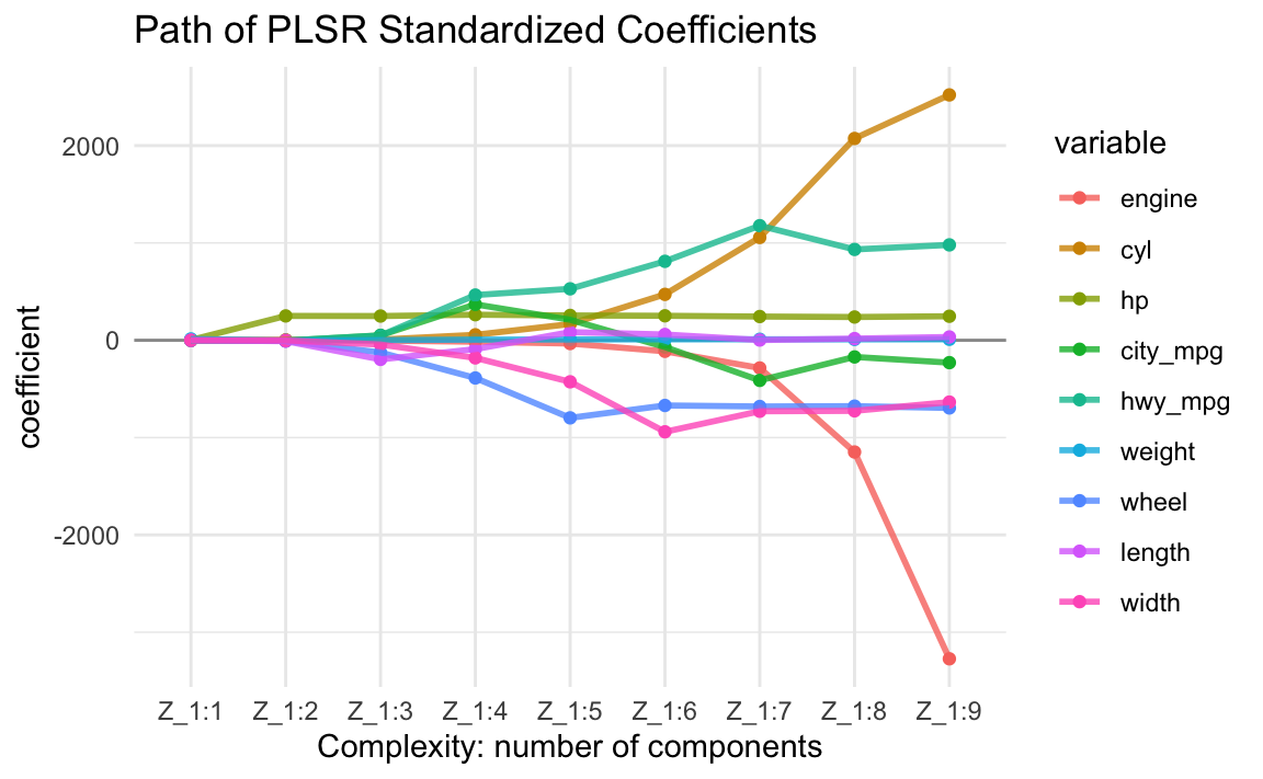
16.4.4 Size of Coefficients
Let’s look at the evolution of the PLS regression coefficients. This is a very interesting plot that allows us to see how the size of the coefficients grow as we add more and more PLS components into the regression equation:
16.5 Selecting Number of PLS Components
The number \(k\) of PLS components to use in PLS Regression is a hyperparameter or tuning parameter. This means that we cannot derive an analytical expression that tells us what the number \(k\) of PCs is the optimal to be used. So how do we find \(k\)? We find \(k\) through resampling methods; the most popular resampling technique being \(K\)-fold cross-validation, although you can use other type of resampling approach. Here’s a description of the steps to be carried out:
Assumet that we have a training data set consisting of \(n\) data points: \(\mathcal{D}_{train} = (\mathbf{x_1}, y_1), \dots, (\mathbf{x_n}, y_n)\). To avoid confusion between the number of PLS components \(k\), and the number of folds \(K\), here we are going to use \(Q = K\) to indicate the index of folds.
Using \(Q\)-fold cross-validation, we (randomly) split the data into \(Q\) folds:
\[ \mathcal{D}_{train} = \mathcal{D}_{fold-1} \cup \mathcal{D}_{fold-2} \dots \cup \mathcal{D}_{fold-Q} \]
Each fold set \(\mathcal{D}_{fold-q}\) will play the role of an evaluation set \(\mathcal{D}_{eval-q}\). Having defined the \(Q\) fold sets, we form the corresponding \(Q\) retraining sets:
- \(\mathcal{D}_{train-1} = \mathcal{D}_{train} \setminus \mathcal{D}_{fold-1}\)
- \(\mathcal{D}_{train-2} = \mathcal{D}_{train} \setminus \mathcal{D}_{fold-2}\)
- \(\dots\)
- \(\mathcal{D}_{train-Q} = \mathcal{D}_{train} \setminus \mathcal{D}_{fold-Q}\)
The cross-validation procedure then repeats the following loops:
- For \(k = 1, 2, \dots, r = rank(\mathbf{X})\)
- For \(q = 1, \dots, Q\)
- fit PLSR model \(h_{k,q}\) with \(k\) PLS-scores on \(\mathcal{D}_{train-q}\)
- compute and store \(E_{eval-q} (h_{k,q})\) using \(\mathcal{D}_{eval-q}\)
- end for \(q\)
- compute and store \(E_{cv_{k}} = \frac{1}{Q} \sum_k E_{eval-q}(h_{k,q})\)
- For \(q = 1, \dots, Q\)
- end for \(k\)
- Compare all cross-validation errors \(E_{cv_1}, E_{cv_2}, \dots, E_{cv_r}\) and choose the smallest of them, say \(E_{cv_{k^*}}\)
- Use \(k^*\) PLS scores to fit the (finalist) PLSR model: \(\mathbf{\hat{y}} = b_1 \mathbf{z_1} + b_2 \mathbf{z_2} + \dots + b_{k^*} \mathbf{z_{k^*}} = \mathbf{Z_{1:k^*}} \mathbf{b_{1:k^*}}\)
- Remember that we can reexpress the PLSR model in terms of the original predictors: \(\mathbf{\hat{y}} = (\mathbf{X} \mathbf{\overset{*}{W}_{1:k^*}}) \mathbf{b_{1:k^*}} = \mathbf{X} \mathbf{\overset{*}{b}_k}\)
Remarks
- PLS regression is somewhat close to Principal Components regression (PCR).
- Like PCR, PLSR involves projecting the response onto uncorrelated components (i.e. linear combinations of predictors).
- Unlike PCR, the way PLS components are extracted is by taking into account the response variable.
- We can conveniently reexpress the solution in terms of the original predictors.
- PLSR is not based on any optimization criterion. Rather it is based on an interative algorithm (which converges)
- Simplicity in its algorithm: no need to invert any matrix, no need to diagonalize any matrix. All you need to do is compute simple regressions. In other words, you just need inner products.
- Missing data is allowed (but you need to modify the algorithm).
- Easily extendable to the multivariate case of various responses.
- Handles cases where we have more predictors than observations (\(p \gg n\)).