6 Gradient Descent

Before moving to the next part of the book which deals with the theory of learning, we want to introduce a very popular optimization technique that is commonly used in many statistical learning methods: the famous gradient descent algorithm.

6.1 Error Surface

Consider the overall error measure of a linear regression problem, for example the mean squared error (\(\text{MSE}\))—or if you prefer the sum of squared errors, which is simply \(\text{SSE} = n \text{MSE}\).

\[ E(\mathbf{y}, \mathbf{\hat{y}}) = \frac{1}{n} \left( \mathbf{b^\mathsf{T} X^\mathsf{T}} \mathbf{X b} - 2 \mathbf{b^\mathsf{T} X^\mathsf{T} y} + \mathbf{y^\mathsf{T}y} \right) \tag{6.1} \]

As we saw in the previous chapter, we can look at such error measure from the perspective of the parameters (i.e. the regression coefficients). From this perspective, we denote this error function as \(E(\mathbf{b})\), making explicit its dependency on the vector of coefficients \(\mathbf{b}\).

\[ E(\mathbf{b}) = \frac{1}{n} ( \underbrace{\mathbf{b^\mathsf{T} X^\mathsf{T}} \mathbf{X b}}_{\text{Quadratic Form}} - \underbrace{ 2 \mathbf{b^\mathsf{T} X^\mathsf{T} y}}_{\text{Linear}} + \underbrace{ \mathbf{y^\mathsf{T}y}}_{\text{Constant}} ) \tag{6.2} \]

As you can tell, \(E(\mathbf{b})\) is a quadratic function with respect to \(\mathbf{b}\). Moreover, \(E(\mathbf{b})\) is a positive semidefinite quadratic form which implies that it is a convex function.

What does this all mean?

For illustration purposes, let’s consider again a linear regression with two inputs \(X_1\) and \(X_2\), and assume that there is no constant term. In this case, the error function \(E(\mathbf{b})\) will generate a convex error surface with the shape of a bowl:

Figure 6.1: Error Surface

In general, with a convex error function, we know that there is a minimum,
and the challenge is to find such value.

Figure 6.2: Error Surface

With OLS we can use direct methods to obtain the minimum. All we need to do is to compute the derivative of the error function \(E(\mathbf{b}\)), set it equal to zero, and find this minimum point \(\mathbf{\overset{*}{b}}\). As you know, assuming that the matrix \(\mathbf{X^\mathsf{T} X}\) is invertible, the OLS minimum is easily calculated as: \(\mathbf{b} = (\mathbf{X^\mathsf{T}X})^{-1} \mathbf{X^\mathsf{T} y}\).

Interestingly, we can also use iterative methods to compute this minimum. The iterative method that we will discuss here is called gradient descent.

6.2 Idea of Gradient Descent

The main idea of gradient descent is as follows: we start with an arbitrary point \(\mathbf{b}^{(0)} = ( b_1^{(0)}, b_2^{(0)} )\) of model parameters, and we evaluate the error function at this point: \(E(\mathbf{b}^{(0)})\). This gives us a location somewhere on the error surface. See figure below.

Figure 6.3: Starting position on error surface

We then get a new vector \(\mathbf{b}^{(1)}\) in a way that we “move down” the surface to obtain a new position \(E(\mathbf{b}^{(1)})\):

Figure 6.4: Begin to move down on error surface

We keep “moving down” the surface, obtaining at each step \(s\) subsequent new vectors \(\mathbf{b}^{(s)}\) that result in an error \(E(\mathbf{b}^{(s)})\) that is closer to the minimum of \(E(\mathbf{b})\).

Figure 6.5: Keep moving down on error surface

Eventually, we should get very, very close to the minimizing point, and ideally, arrive at the minimum \(\mathbf{\overset{*}{b}}\).

One important thing to always keep in mind when dealing with minimization (and maximization) problems is that, in practice, we don’t get to see the surface. Instead, we only have local information at the current point we evaluate the error function.

Here’s a useful metaphor: Imagine that you are on the top a mountain (or some similar landscape) and your goal is to get to the bottom of the valley. The issue is that it is a foggy day (or night), and the visibility conditions are so poor that you only get to see/feel what is very near you (a couple of inches around you). What would you do to get to the bottom of the valley? Well, you start touching your surroundings trying to feel in which direction the slope of the terrain goes down. The key is to identify the direction in which the slope gives you the steepest descent. This is the conceptual idea behind optimization algorithms like gradient descent.

6.3 Moving Down an Error Surface

What do we mean by “moving down the error surface”? Well, mathematically, this means we generate the new vector \(\mathbf{b}^{(1)}\) from the initial point \(\mathbf{b}^{(0)}\), using the following formula:

\[ \mathbf{b}^{(1)} = \mathbf{b}^{(0)} + \alpha \mathbf{v}^{(s)} \tag{6.3} \]

As you can tell, in addition to the values of parameter vectors \(\mathbf{b}^{(0)}\) and \(\mathbf{b}^{(1)}\), we have two extra ingredients: \(\alpha\) and \(\mathbf{v}^{(s)}\).

We call \(\alpha\) the step size. Intuitively, \(\alpha\) tells us how far down the surface we are moving. In turn, \(\mathbf{v}^{(s)}\) is the vector indicating the direction in which we need to move. Because we are interested in this direction, we can simply consider \(\mathbf{v}^{(s)}\) to be a unit vector. We will discuss how to find the direction of \(\mathbf{v}^{(s)}\) in a little bit. Right now let’s just focus on generating new vectors in this manner:

\[\begin{align*} \mathbf{b}^{(2)} & = \mathbf{b}^{(1)} + \alpha \mathbf{v}^{(1)} \\ \mathbf{b}^{(3)} & = \mathbf{b}^{(2)} + \alpha \mathbf{v}^{(2)} \\ \vdots & \hspace{10mm} \vdots \\ \mathbf{b}^{(s+1)} & = \mathbf{b}^{(s)} + \alpha \mathbf{v}^{(s)} \tag{6.4} \end{align*}\]

Note that we are assuming a constant step size \(\alpha\); that is, note that \(\alpha\) remains the same at each iteration. We should say that there are more sophisticated versions of gradient descent that allow a variable step size, however we will not consider that case. As we can see in the series of figures above, the direction in which we travel will change at each step of the process. We will also see this mathematically in the next subsection.

6.3.1 The direction of \(\mathbf{v}\)

How do we find the direction of \(\mathbf{v}^{(s)}\)? Consider the gradient of our error function. The gradient always points in the direction of steepest ascent (i.e. largest positive change). Hence, we want to travel in the exact opposite direction of the gradient.

Let’s “prove” this mathematically. In terms of the error function itself, what does it mean for our vectors \(\mathbf{b}^{(s+1)}\) to be “getting closer” to the minimizing point? Well, it means that the error at point \(\mathbf{b}^{(s+1)}\) is less than the error at point \(\mathbf{b}^{(s)}\). Hence, we examine \(\Delta E_{\mathbf{b}}\), the difference between the errors at these two points:

In order for our vector \(\mathbf{b}^{(s+1)}\) to be closer to the minimizing point, we want this quantity \(\Delta E_{\mathbf{b}}\) to be as negative as possible. To find the vector \(\mathbf{v}^{(s)}\) that makes this true, we apply Taylor series expansion of \(E(\mathbf{b}^{(s)} + \alpha \mathbf{v}^{(s)})\). Doing so, we obtain:

\[\begin{align*} \Delta E_{\mathbf{b}} &= E\big( \mathbf{b}^{(s)} \big) + \nabla E\big( \mathbf{b}^{(s)} \big)^{\mathsf{T}} \big(\alpha \mathbf{v}^{(s)} \big) + O \big( \alpha^2 \big) - E\big( \mathbf{b}^{(s)} \big) \\ & = \alpha \hspace{1mm} \nabla E \big( \mathbf{b}^{(s)} \big)^{\mathsf{T}} \mathbf{v}^{(s)} + O(\alpha^2) \tag{6.6} \end{align*}\]

where \(O(\alpha^2)\) denotes those terms of order 2 or greater in the series expansion.

We will focus our attention on the series expansion of just one term, and ignore the higher order terms comprised by \(O(\alpha^2)\). In other words, we will focus on the first-order term: \(\alpha \hspace{1mm} \nabla E \big( \mathbf{b}^{(s)} \big)^{\mathsf{T}} \mathbf{v}^{(s)}\). Notice that this term involves the inner product between the gradient and the unit vector \(\mathbf{v}^{(s)}\), that is:

\[ [ \nabla E(\mathbf{b}^{(s)})]^{\mathsf{T}} \mathbf{v}^{(s)} \]

For notational convenience, let us (temporarily) drop the superindex \((s)\), and let’s denote the gradient as \(\mathbf{u}\):

\[ \mathbf{u} : = \nabla E ( \mathbf{b}^{(s)} ) \tag{6.7} \]

In this way, we need to examine the inner product: \(\mathbf{u^\mathsf{T}v}\). We can consider three prototypical cases with respect to the orientation of \(\mathbf{v}\) and \(\mathbf{u}\): either antiparallel, parallel, or orthogonal.

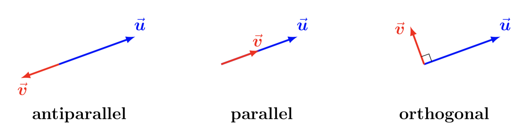
Figure 6.6: Three prototypical cases

When both vectors are parallel, \(\mathbf{u} \parallel \mathbf{v}\) (i.e. the second case above), then \(\mathbf{u}^\mathsf{T}\mathbf{v} = \| \mathbf{u} \|\). Recall that we are assuming \(\mathbf{v}\) to be a unit vector.
When both vectors are antiparallel, \(\mathbf{u} \not\parallel \mathbf{v}\) (i.e. the first case above), then \(\mathbf{u}^\mathsf{T} \mathbf{v} = - \| \mathbf{u} \|\).
When both vectors are orthogonal, \(\mathbf{u} \perp \mathbf{v}\), then \(\mathbf{u}^\mathsf{T} \mathbf{v} = 0\).

Therefore, in any of the three cases, we have that

\[ \mathbf{u}^\mathsf{T} \mathbf{v} \geq - \left\| \mathbf{u} \right\| \tag{6.8} \]

This means that the least we can get is \(- \left\| \mathbf{u} \right\|\), which occurs when \(\mathbf{v}\) is in the opposite direction of \(\mathbf{u}\).

Hence, recalling that \(\mathbf{u} := \nabla E(\mathbf{b}^{(s)})\), we can plug this result into our error computation to obtain:

\[\begin{align*} \Delta E_{\mathbf{b}} & := E\big( \mathbf{b}^{(s + 1)} \big) - E\big( \mathbf{b}^{(s)} \big) \\ & = E \big( \mathbf{b}^{(s)} + \alpha \mathbf{v}^{(s)} \big) - E\big( \mathbf{b}^{(s)} \big) \\ & = \alpha \hspace{1mm} \nabla E \big( \mathbf{b}^{(s)} \big)^{\mathsf{T}} \mathbf{v}^{(s)} + O(\alpha^2) \\ & \geq - \alpha \left\| \nabla E\big( \mathbf{b}^{(s)} \big) \right\| \tag{6.9} \end{align*}\]

Thus, to make \(\Delta E_{\mathbf{b}}\) as negative as possible, we should take \(\mathbf{v}^{(s)}\) parallel to the opposite direction of the gradient.

The Moral: We want the following:

\[ \mathbf{v}^{(s)} = - \frac{\nabla E(\mathbf{b}^{(s)}) }{\left\| \nabla E(\mathbf{b}^{(s)}) \right\| } \tag{6.10} \]

which means we want to move in the direction opposite to that of the gradient. Notice that we divide by the norm because we previously defined \(\mathbf{v}^{(s)}\) to be a unit vector. This normalization is very beningn, and we don’t really need while implement gradient descent computationally because it will be “passed to” the step size \(\alpha\).

This also reveals the meaning behind the name gradient descent; we are descending in the direction opposite to the gradient of the error function.

6.4 GD Algorithm for Linear Regression

We present the full algorithm for gradient descent in the context of regression under both flavors: 1) using vector-matrix notation, and 2) using pointwise (or element-wise) notation.

6.4.1 GD Algorithm in vector-matrix notation

The starting point is the formula for \(E(\mathbf{b})\)

\[\begin{align*} E(\mathbf{b}) & = \frac{1}{n} \left( \mathbf{y} - \mathbf{X} \mathbf{b} \right)^{\mathsf{T}} \left( \mathbf{y} - \mathbf{X} \mathbf{b} \right) \\ \\ & = \frac{1}{n} \left( \mathbf{b}^\mathsf{T} \mathbf{X}^\mathsf{T} \mathbf{X} \mathbf{b} - 2 \mathbf{b}^\mathsf{T} \mathbf{X}^\mathsf{T} \mathbf{y} + \mathbf{y}^\mathsf{T} \mathbf{y} \right) \\ \tag{6.11} \end{align*}\]

We can find a closed form for its gradient \(\nabla E(\mathbf{b})\):

\[\begin{align*} \nabla E(\mathbf{b}) & = \frac{1}{n} \left( 2 \mathbf{X}^\mathsf{T} \mathbf{X} \mathbf{b} - 2 \mathbf{X}^\mathsf{T} \mathbf{y} \right) \\ &= \frac{2}{n} \mathbf{X}^\mathsf{T} (\mathbf{Xb} - \mathbf{X^\mathsf{T}y}) \tag{6.12} \end{align*}\]

Algorithm

Initialize a vector \(\mathbf{b}^{(0)} = \left( b_{0}^{(0)}, b_{1}^{(0)}, \dots, b_{p}^{(0)} \right)\)

Repeat the following over \(s\) (starting with \(s = 0\)), until convergence:

\[\begin{align*} \mathbf{b}^{(s+1)} &= \mathbf{b}^{(s)} - \alpha \ \nabla E \big( \mathbf{b}^{(s)} \big) \\ &= \mathbf{b}^{(s)} - \alpha \left[ \frac{2}{n} \ \mathbf{X}^\mathsf{T} (\mathbf{Xb}^{(s)} - \mathbf{X^\mathsf{T}y}) \right] \tag{6.13} \end{align*}\]

When there is little change between \(\mathbf{b}^{(k + 1)}\) and \(\mathbf{b}^{(k)}\) (for some integer \(k\)), the algorithm will have converged and \(\mathbf{b}^{*} = \mathbf{b}^{(k+1)}\).

6.4.2 GD algorithm in pointwise notation

The above formula involves the columns point of view. However, we can also find a formula from the row’s perspective (i.e. in pointwise notation):

\[\begin{align*} E(\mathbf{b}) & = \frac{1}{n} \sum_{i = 1}^{n} \left( y_i - \mathbf{b}^\mathsf{T} \mathbf{x_i} \right)^2 = \frac{1}{n} \sum_{i=1}^{n} \left( y_i - \hat{y}_i \right)^2 \\ & = \frac{1}{n} \sum_{i=1}^{n} \left( y_i - b_0 x_{i0} - b_1 x_{i1} - \dots - b_{j} x_{ij} - \dots - b_{p} x_{ip} \right)^2 \\ \tag{6.14} \end{align*}\]

The partial derivative with respect to \(b_j\) is:

\[\begin{align*} \frac{\partial E(\mathbf{b})}{\partial b_j} & = - \frac{2}{n} \sum_{i=1}^{n} \left( y_i - b_0 x_{i0} - \dots - b_{j} x_{ij} - \dots - b_{p} x_{ip} \right) x_{ij} \\ & = - \frac{2}{n} \sum_{i=1}^{n} \left( y_i - \mathbf{b}^{\mathsf{T}} \mathbf{x_i} \right) x_{ij} \tag{6.15} \end{align*}\]

This will be a better formula to use in our iterative algorithm, described below.

Algorithm

Initialize a vector \(\mathbf{b}^{(0)} = \left( b_{0}^{(0)}, b_{1}^{(0)}, \dots, b_{p}^{(0)} \right)\)

Repeat the following over \(s\) (starting with \(s = 0\)), until convergence:

\[ b_{j}^{(s+1)}:= b_{j}^{(s)} + \alpha \cdot \frac{2}{n} \sum_{i=1}^{n} \left( y_i - \left[\mathbf{b}^{(s)}\right]^{\mathsf{T}} \mathbf{x_i} \right) x_{ij} \tag{6.16} \]

for all \(j = 0, \dots, p\) simultaneously.

In more compact notation,

\[ b_{j}^{(s+1)} = b_{j}^{(s)} + \alpha \cdot \frac{\partial }{\partial b_j} E(\mathbf{b}^{(s)}) \tag{6.17} \]

Store these elements in the vector \(\mathbf{b}^{(s+1)} = \left( b_{0}^{(s+1)} , b_{1}^{(s+1)} , \dots, b_{p}^{(s+1)} \right)\)

When there is little change between \(\mathbf{b}^{(k + 1)}\) and \(\mathbf{b}^{(k)}\) (for some integer \(k\)), the algorithm will have converged and \(\mathbf{b}^{*} = \mathbf{b}^{(k+1)}\).

Note that in the algorithm, we have dropped the condition that \(\mathbf{v}\) is a unit vector. Indeed, if you look on the Wikipedia page for Gradient Descent the algorithm listed there also omits the unit-length condition.