29 Performance of Classifiers
Now that we have described several classification methods, it is time to discuss the evaluation of their predictive performance. Specifically, the pertaining question is: How do we measure the performance of a classifier?
29.1 Classification Error Measures
Recall that, in supervised learning, we are interested in obtaining models that give accurate predictions. At the conceptual level we need some mechanism to quantify how different a fitted model \(\widehat{f}\) is from the target function \(f\):
\[ \widehat{f} \text{ -vs- } f \]
This means that we need an error function that summarizes the total amount of error, also referred to as the Overall Measure of Error:
\[ \text{Overall Measure of Error:} \quad E(\widehat{f},f) \]
The typical way in which an overall measure of error is defined is in terms of individual or pointwise errors \(err_i(\hat{y}_i, y_i)\) that quantify the difference between an observed value \(y_i\) and its predicted value \(\hat{y}_i\). Usually, most overall errors aggregate pointwise errors into a single measure:
\[ E(\widehat{f},f) = \text{measure} \left( \sum err_i(\hat{y}_i, y_i) \right ) \tag{29.1} \]
In a classification setting we still have response observations \(y_i\) and predicted values \(\hat{y}_i\); we still want a way to compare \(y_i\) versus \(\hat{y}_i\); and we still need an overall measure of error.
29.1.1 Errors for Binary Response
The starting point involves finding a pointwise error function. Assuming that we have a binary response, that is \(y_i \in \{0, 1\}\), and assuming also that the predicted values are binary as well, \(\hat{y}_i \in \{0, 1\}\), then we could use the absolute error as a pointwise error measure:
\[ \left| y_i - \hat{y}_i \right| = \begin{cases} 0 & \text{if } y_i = \hat{y}_i \\ & \\ 1 & \text{if } y_i \neq \hat{y}_i \\ \end{cases} \tag{29.2} \]
or we could also use squared error:
\[ (y_i - \hat{y}_i)^2 = \begin{cases} 0 & \text{if agree} \\ & \\ 1 & \text{if disagree} \\ \end{cases} \tag{29.3} \]
Again, keep in mind that the above error functions are valid as long as the predictions are binary, \(\hat{y}_i \in \{0, 1\}\), which is not always the case for all classifiers.
Now, suppose we still had binary data but instead we encoded our data so that \(y_i \in \{-1, 1\}\). What kind of pointwise error measure should we use? If we used squared error, we would get the following:
\[ (y_i - \hat{y}_i)^2 = \begin{cases} 0 & \text{if agree} \\ & \\ 4 & \text{if disagree} \\ \end{cases} \tag{29.4} \]
Alternatively, under the same assumption that \(y_i \in \{-1, 1\}\), we could consider the product between the observed response and its predicted value:
\[ y_i \times \hat{y}_i = \begin{cases} +1 & \text{if agree} \\ & \\ -1 & \text{if disagree} \\ \end{cases} \tag{29.5} \]
The point that we are trying to make is that there are many different choices for pointwise error measures.
Perhaps the most common option of pointwise error is the binary error, defined to be:
\[ [\![ \hat{y}_i \neq y_i ]\!] \to \begin{cases} 0 \ (\text{or FALSE}) & \text{if agree} \\ & \\ 1 \ (\text{or TRUE}) & \text{if disagree} \\ \end{cases} \tag{29.6} \]
This type of error function is adequate for classification purposes, and it works well for the case in which we have a binary response, as well as when we have a response with more than two categories. Moreover, averaging these binary errors over our observations yields the classification error rate:
\[ \text{classif. error rate:} \quad \frac{1}{n} \sum_{i=1}^{n} [\![ \hat{y}_i \neq y_i ]\!] \tag{29.7} \]
29.1.2 Error for Categorical Response
Now suppose we have a categorical response with more than two categories. For example, \(y_i \in \{a, b, c, d\}\). For illustrative purposes, consider the following data with hypothetical predictions:
\[ \begin{array}{c|ccccc} y & a & b & c & d & b \\ \hline \hat{y} & a & a & c & d & c \\ \hline & \checkmark & \times & \checkmark & \checkmark & \times \\ \end{array} \]
here the symbol \(\checkmark\) denotes agreement between the observed values and the predicted values. In this case, it makes sense to use the binary error as our pointwise error measure previously defined:
\[ [\![ \hat{y}_i \neq y_i ]\!] \to \begin{cases} 0 \ (\text{or FALSE}) & \text{if agree} \\ & \\ 1 \ (\text{or TRUE}) & \text{if disagree} \\ \end{cases} \tag{29.8} \]
As in the binary-response case discussed in the previous section, averaging these pointwise errors over our observations yields the misclassification error rate:
\[ \frac{1}{n} \sum_{i=1}^{n} [\![ \hat{y}_i \neq y_i ]\!] \tag{29.9} \]
This overall measure of error is the one that we’ll use in this book, unless mentioned otherwise.
29.2 Confusion Matrices
Regardless of the pointwise error measure to be used, it is customary to construct a confusion matrix. This matrix is simply a crosstable representation of the number of agreements and disagreements between the observed response values \(y_i\) and the corresponding predicted values \(\hat{y}_i\).
In the binary-response case with \(0-1\) encoding, \(y_i \in \{0, 1\}\), the confusion matrix has the following format:

Any entry in this matrix contains information about how our predicted classes compare with the observed classes. For example, the entry in row-1 and column-1 represents the number of observations that are correctly classified as being of class \(0\). In contrast, the entry in the row-2 and column-1 indicates the number of observations that are classified as \(1\) when in fact they are actually of class \(0\). As such, the off-diagonal entries represent observations that are misclassified.
In general, for a response with more than 2 categories, for example \(K=4\), the confusion matrix will take the form of a \(K \times K\) matrix:

The way we read this crosstable is the same as in the binary-response case. For example, the number in the entry of row-1 and column-2 represents the number of observations that are classified as being of class \(a\) when in fact they are actually of class \(b\). Likewise, the off-diagonal entries represent observations that are misclassified. We can calculate the misclassification error from the confusion matrix using the following formula:
\[\begin{align*} \text{Misclassification Error} &= 1 - \frac{\sum (\text{all cells in diagonal}) }{n} \\ &= \frac{\sum (\text{all cells off-diagonal}) }{n} \\ &= \frac{1}{n} \sum_{i=1}^{n} [\![ \hat{y}_i \neq y_i ]\!] \tag{29.10} \end{align*}\]
In this way, the “ideal” confusion matrix of a perfect classifier is one that is completely diagonal, with all off-diagonal entries equal to \(0\). The higher the off-diagonal entries, the worse our model is performing.
29.3 Binary Response Example
Consider an application process for a potential customer that is interested in some financial product.

Our hypothetical customer approaches a certain bank and goes through the process to get approval for a financial product like:
- Savings or Checking Accounts
- Credit Card
- Car Loan
- Mortgage Loan
- Certificate of Deposit (CD)
- Money Market Account
- Retirement Account (e.g. IRA)
- Insurance policy
- etc
For each of these applications, there will be some series of questions the customer needs to answer. Here’s a screenshot of a typical online application form for a credit card (btw: as of this writing, one of the book authors owns such credit card, but he’s not affiliated with the brand):
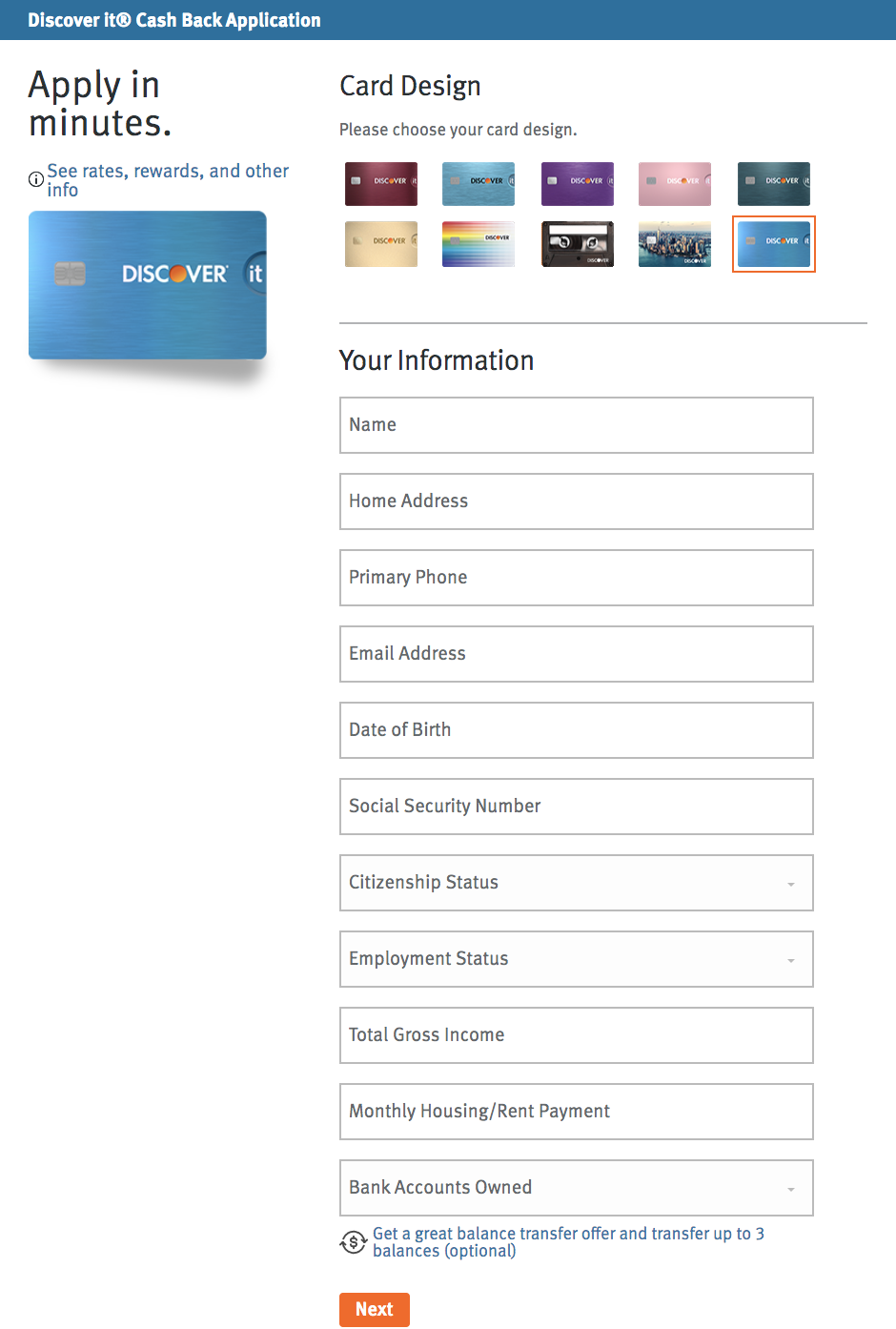
Using some or all of the descriptors for a customer, we want a model \(f\) that takes the answers to these questions, denoted as \(\mathbf{x_i}\), and spits out either \(\text{accept}\) or \(\text{reject}\). Pictorially:
\[ \mathbf{x_i} \to \boxed{\hat{f}} \to \hat{y}_i = \begin{cases} \text{accept application} \\ & \\ \text{reject application} \\ \end{cases} \tag{29.11} \]
Now, given past data on acceptances and rejections of previous customers, the confusion matrix will have the following four types of entries:

The entries in the digonal are correct or “good” predictions, whereas the off-diagonal entries correspond to classification errors. Notice that we have two flavors of misclassifications. One of them is “false reject” when a good customer is incorrectly rejected. The other one is “false accept” when a bad customer is incorrectly accepted.
In an ideal situation, we would simultaneously minimize the false acceptance and false rejection rates. However, as with everything else in Machine Learning, there is a tradeoff; in general, minimizing false acceptance rates increases false rejection rates, and vice-versa. We discuss this issue in the last section of this chapter.
One interesting aspect in classification has to do with the importance of classification errors. In our hypothetical example: Are both types of errors, “false accept” and “false reject”, equally important? As you can imagine, there may be situations in which a false acceptance is “worse” (in some way) than a false rejection, and vice versa. We explore these considerations with a couple of examples in the next sections.
29.3.1 Application for a Checking Account
Let’s further investigate the different types of errors that may occur in a classification scenario. For instance, let’s consider an application process for a financial product like a checking (or a savings) account.

To make things more interesting, suppose that one bank has a promotion of a cash bonus when someone opens a new checking account with them.
Here’s a screenshot of a typical online application form for a checking account:
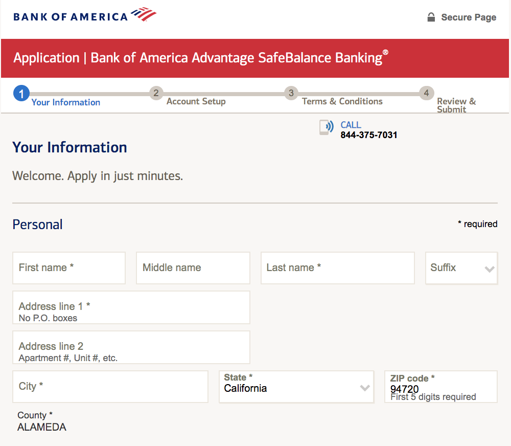
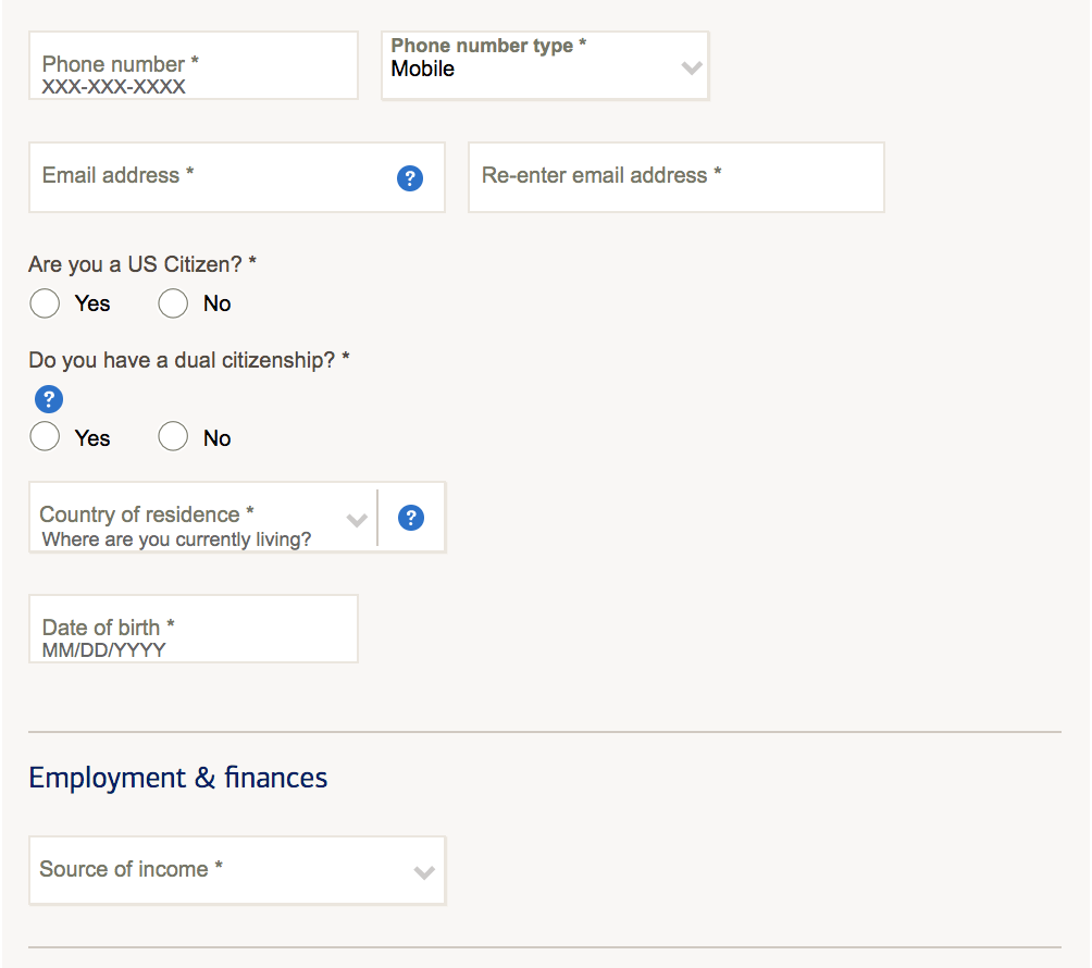
As we mention above, using some or all of the descriptors for a customer, we want a model \(f\) that takes the answers to the questions in the application form, denoted as \(\mathbf{x_i}\), and produces an output:
\[ \mathbf{x_i} \to \boxed{\hat{f}} \to \hat{y}_i = \begin{cases} \text{accept} \\ & \\ \text{reject} \\ \end{cases} \tag{29.12} \]
The format of the confusion matrix will be something like this:

As you can tell, we have two types of errors. The first kind of error is a false rejection. This occurs when a customer fills out an application for a checking account, and despite the fact that they are theoretically eligible to open such account, this customer is rejected.
The second kind of error is a false acceptance; that is, a customer who is (theoretically) an unsuited customer for the bank, still gets approved to open an account.
Which type of error is worse from the bank’s point of view?
The answer is: a false rejection! This is because the “good” customer would likely be able to go across the street and open up an account at the rival bank; that is, the initial bank has lost a potential customer. As for the false accept, this is a type of error that the bank can better tolerate, and the lucky customer will receive the cash bonus.
Hence, when constructing the confusion matrix, we might want to assign different penalties to the different errors. For example we can give a penalty of 5 for a false reject, and a penalty of 1 for a false accept. We do this because the false reject is considered to be more costly than a false accept.

Note that the values 1 and 5 were somewhat arbitrary; the actual values are less important as the relative magnitude of them (for example we could have just as easily used \(20\) and \(50\), respectively, instead). Obviously the amount of penalty values depend on expertise information, and will vary from one classification problem to another.
29.3.2 Application for a Loan
Now, suppose that the application process in question is for a loan (e.g. mortgage loan, or car loan).

The two types of errors still stand: false rejection and false acceptance.
Like in the previous example about the checking account, we also have the same two types of errors:
False Rejection: This occurs when a customer fills out an application for a loan, and despite the fact that they are theoretically eligible to borrow money, this customer is rejected.
False Acceptance: This occurs when a customer who is (theoretically) an unsuited customer for the bank, still gets approved to borrow money.
Same question: which error is more costly (from the bank’s point of view)? If you think about it, now the two errors have different interpretations and consequences:
With false reject, the bank loses money that they could have gathered through interest from the customer.
With false acceptance, the bank loses money because the customer will ultimately default and not pay back the loan.
It shouldn’t be too difficult to notice that a false acceptance is worse than a false rejection. If the bank grants a loan to someone who won’t be able to pay it back in the long run, the bank will lose money (likely more money than they would have gained through interest from somebody who could have paid their loan). Hence, we might assign the following penalties:

We should mention that the penalties assigned to each type of error is not an analytic question but rather an application domain question. What penalty we use depends on a case by case. Likewise, there is no inherent merrit in choosing one error penalty over another. In summary, the combination of the error measure and the penalties, it’s something that should be specified by the user.
29.4 Decision Rules and Errors
Another aspect that we need to discuss involves dealing with classifiers that produce a class assignment probability, or a score that is used to make a decision. A typical example is logistic regression.
Recall that in logistic regression we model the posterior probabilities of the response given the data as:
\[ Prob(y_i \mid \mathbf{x_i}, \mathbf{b}) = \begin{cases} h(\mathbf{x_i})& \textsf{for } y_i = 1 \\ & \\ 1 - h(\mathbf{x_i}) & \textsf{for } y_i = 0 \\ \end{cases} \tag{29.13} \]
where \(h()\) denotes the logistic function \(\phi()\):
\[ h(\mathbf{x}) = \phi(\mathbf{b^\mathsf{T} x}) \tag{29.14} \]
In this case, logistic regression provides both ways of handling the output, with the probability \(P(y \mid \mathbf{x})\) or with a score given by the linear signal \(s = \mathbf{b^\mathsf{T} x}\).
Suppose that \(y = 1\) corresponds to \(\text{accept}\) and \(y = 0\) corresponds to \(\text{reject}\). If we look at the graph of \(P(y)\) and the logistic function of the linear signal, we can get a picture like this:

\[ P(y = 1) = \frac{e^{\mathbf{b^\mathsf{T} x}} }{1 + e^{\mathbf{b^\mathsf{T} x}} } \tag{29.15} \]
Now, suppose we have three individuals \(A\), \(B\) and \(C\) with the following acceptance probabilities:
\[ P(\text{accept}_A) = 0.9; \quad P(\text{accept}_B) = 0.1; \quad P(\text{accept}_C) = 0.5 \tag{29.16} \]
To classify these, we would need to introduce some sort of cutoff \(\tau\) so that our decision rule is
\[ \text{decision rule} = \begin{cases} \text{accept} & \text{if } P(\text{accept}) > \tau \\ & \\ \text{reject} & \text{otherwise} \\ \end{cases} \tag{29.17} \]
Where should we put \(\tau\)? The default options is to set it at \(0.5\):

Going back to the example of a loan application, we know that a false accept is a more dangerous type of error than a false reject. Setting \(\tau = 0.5\) doesn’t really make too much sense from the bank’s perspective, if what we want is to prevent accepting customers that will eventually default on their loans. It would make more sense to set \(\tau\) to a value much higher than 0.5; for example, 0.7:

Think of this a “raising the bar” for customer applications. The bank will be more strict in approving customers applications, safeguarding against the “worst” type of error (in this case, false acceptances).
For comparison purposes, let’s momentarilly see what could happen if we set \(\tau = 0.3\). A threshold with this value would increase the number of false acceptance.

The bank would be “lowering the bar”, being less strict with the profile of accepted customers. Consequently, the bank would be running a higher risk by giving loans to customers that may be more likely to default.
Note that the confusion matrix will change depending on the value of \(\tau\) we pick.
29.5 ROC Curves
So, then, what value of \(\tau\) should we pick? To answer this question, we will use a ROC curve which stands for Receiving Operating Characteristic curve. Keep in mind that ROC curves are only applicable to binary responses. We introduce the following notations in a confusion matrix:

The general form of the confusion matrix is the same. The entries on the diagonal have to do with observations correctly classified. In turn, the off-diagonal entries have to do observations incorrectly classified. The difference is the way in which categories are encoded: \(\text{accept}\) is now encoded as positive, while \(\text{reject}\) is encoded as negative. By the way, this encoding is arbitrary, and you can choose to label \(\text{accept}\) as negative, and \(\text{reject}\) as positive.
A more common notation involves further abbreviating each of the names in the cells of a confusion matrix as follows:

where \(\text{TP}\) stands for “true positive,” \(\text{FP}\) stands for “false positive,” \(\text{FN}\) stands for “false negative,” and \(\text{TN}\) stands for “true negative.” With these values, we can obtain the following rates.
We define the True Positive Rate (\(\text{TPR}\); sometimes called the sensitivity) as
\[ \textsf{sensitivity:} \quad \mathrm{TPR} = \frac{\text{TP}}{\text{TP} + \text{FN}} \tag{29.18} \]
Notice that TPR can be regarded as a conditional probability:
\[ \text{TPR} \quad \longleftrightarrow \quad P(+\hat{y} \mid +y) \tag{29.19} \]
Similarly, we define the True Negative Rate (\(\text{TNR}\); sometimes called the specificity) as
\[ \textsf{specificity:} \quad \mathrm{TNR} = \frac{\text{TN}}{\text{TN} + \text{FP}} \tag{29.20} \]
As with TPR, we can also regard TNR as a conditional probability:
\[ \text{TNR} \quad \longleftrightarrow \quad P(-\hat{y} \mid -y) \tag{29.21} \]
Additionally, we can also get the corresponding False Negative Rate (FNR) defined as one minus sensitivity:
\[ \mathrm{FNR} = 1 - \text{TPR} = \frac{\text{FN}}{\text{TP} + \text{FN}} \tag{29.22} \]
as well as the False Positive Rate (FPR) defined as one minus specificity:
\[ \mathrm{FPR} = 1 - \text{TNR} = \frac{\text{FP}}{\text{TN} + \text{FP}} \tag{29.23} \]
Ideally, we would like to have a classifier or decision rule that simultaneously minimizes both the false acceptance and false rejection rates. However, there is a tradeoff; in general, minimizing false acceptance rates increases false rejection rates, and vice-versa. Why? Because increasing the sensitivity of a classifier results in more observations being predicted as positive.
Returning to the loan application example, and assuming again that \(\text{acceptance}\) is the positive level, sensitivity measures how often the accepted customers in the test set were actually classified as accepted.
29.5.1 Graphing ROC curves
Now that we have introduced the required notation and terminology commonly employed with Receiver Operating Characteristic curves, let’s properly describe this graphic tool.
The ROC curve is one visual tool used to measure the performance of a two-class classifier that uses prediction scores or discriminant functions. The ingredients to plot the ROC curve are True Positive Rate (sensitivity) and False Positive Rate (1 - specificity), for a set of thresholds \(\tau\) used to convert classification scores into predicted responses. To be more precise, a ROC curve is used to show in a visual way the tradeoff between sensitivity and specificity for every possible cut-off or threshould value \(\tau\), for a binary classification score.

Figure 29.1: Example of a ROC Curve
In addition, the area under the ROC curve gives an idea about the benefit of using the decision rule under consideration.
Example
The following figure shows the ROC curves for two discriminant analysis classifiers applied to a simulated data set with two predictors and a two-class response. One of the classifiers is a linear discriminant model (LDA), while the other one is a quadratic discriminant model (QDA). Given a candidate threshold value \(\tau\), the TPR and FPR are graphed against each other. With a large set of thresholds, graphed pairs of TPR and FPR result in a ROC curve.
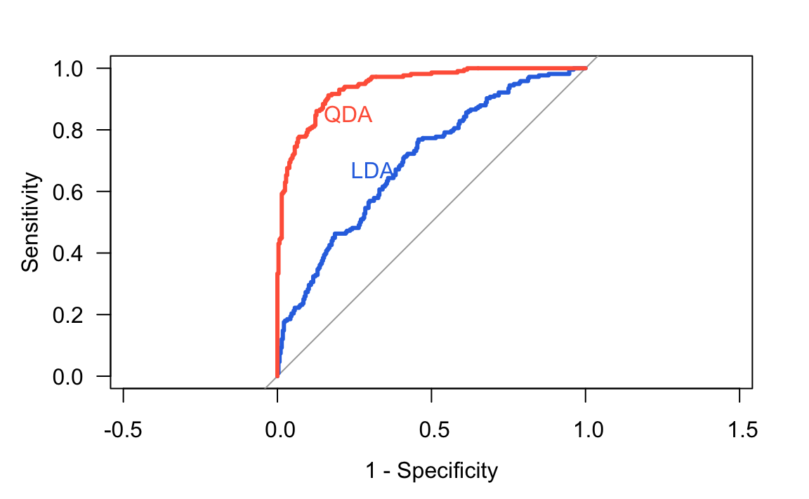
In the figure above, the ROC curve associated to the QDA indicates that this method has better sensitivity and specificity performance than LDA.
One of the purposes of the plot is to give us guidance for selecting a threshold that maximizes the tradeoff between sensitivity and specificity. The best threshold is the one that has the highest sensitivity (TPR) together with the lowest FPR.
The following diagram depicts three possible ROC curve profiles, with a data set of \(n=100\) individuals belonging to two classes of equal size. The left frame shows a ROC cruve from a classifier that produces perfect classifications. This is the best possible ideal scenario. The frame in the middle shows a ROC curve that coincides with the diagonal (dashed line) indicating that the classifier has no discriminant capacity, and is no better than classifying observations at random (e.g. assign classes flipping a coin). Finally, the frame on the right illustrates another extreme case in which the classifier has perfect misclassification performance; this is the worst possible scenario for a classifier.
