32 Hierarchical Clustering
The idea behind hierarchical clustering is to find nested partitions. There are two approaches:
Agglomerative Methods: this is the method we will discuss below.
Divisive Methods: we will not discus this method, however one can think of it as the opposite of agglomerative methods.
32.1 Agglomerative Methods
Agglomerative Hierarchical Clustering (AHC) produce sequences of nested partitions of increasing within-cluster heterogeneity.
Distance and Dissimilarity
As with \(K\)-means, we still need a notion of distance between two observations: this notion could be a distance metric, or a measure of dissimilarity or proximity.
Metric distances satisfy the following properties:
\(d(\mathbf{x_i}, \mathbf{x_\ell}) \geq 0 \quad \textsf{(non-negativity)}\)
\(d(\mathbf{x_i}, \mathbf{x_i}) = 0 \quad \textsf{(reflexivity)}\)
\(d(\mathbf{x_i}, \mathbf{x_\ell}) = d(\mathbf{x_\ell}, \mathbf{x_i}) \quad \textsf{(symmetry)}\)
\(d(\mathbf{x_i}, \mathbf{x_\ell}) \leq d(\mathbf{x_i}, \mathbf{x_k}) + d(\mathbf{x_k}, \mathbf{x_\ell}) \quad \textsf{(triangle inequality)}\)
In turn, dissimilarities satisfy the following three properties:
\(d(\mathbf{x_i}, \mathbf{x_\ell}) \geq 0 \quad \textsf{(non-negativity)}\)
\(d(\mathbf{x_i}, \mathbf{x_i}) = 0 \quad \textsf{(reflexivity)}\)
\(d(\mathbf{x_i}, \mathbf{x_\ell}) = d(\mathbf{x_\ell}, \mathbf{x_i}) \quad \textsf{(symmetry)}\)
Distance of clusters
We also need another type of distance: this one will be used to measure how different two clusters are.
Minimum Distance:
- Also known as single linkage or nearest neighbor.
- Sensitive to the ``chain effect’’ (or chaining): if two widely separated clusters are linked by a chain of individuals, they be grouped together.
Maximum distance:
- Also known as complete linkage or farthest-neighbor technique.
- Tends to generate clusters of equal diameter.
- Sensitive to outliers.
Mean Distance:
- Also known as average linkage.
- Intermediate between the minimum distance and the maximum distance methods.
- Tends to produce clusters having similar variance.
Ward method:
- Matches the purpose of clustering most closely.
- Ward distance defined as the reduction in between-cluster sum of squares.
The following diagram illustrates two clusters with several individuals and their corresponding centroids; listing the common distances between clusters:

Figure 32.1: Aggregation Criteria
Agglomerative Algorithms
The general form of an agglomerative algorithm is as follows:
The initial clusters are the observations.
The distances between clusters are calculated.
The two clusters which are closest together are merged and replaced with a single cluster.
We start again at step 2 until there is only one cluster, which contains all the observations.
The sequence of partitions is presented in what is known as a tree diagram also known as dendrogram.
This tree can be cut at a greater or lesser height to obtain a smaller or larger number of clusters.
The number of clusters can be chosen by optimizing certain statistical quality criteria. The main criterion is the loss of between-cluster sum of squares.
32.2 Example: Single Linkage
Let’s see a toy example. Suppose we have 5 individuals: \(\textsf{a}, \textsf{b}, \textsf{c}, \textsf{d},\) and \(\textsf{e}\), and two variables \(x\) and \(y\), as follows:
   x  y
a  1  4
b  5  4
c  1  3
d  1  1
e  4  3
If we used the squared-euclidean distance as our distance measure, we obtain a matrix of distances like:
    a   b   c   d   e
a   0  16   1   9  10
b  16   0  17  25   2
c   1  17   0   4   9
d   9  25   4   0  13
e  10   2   9  13   0
Here’s a scatterplot of the data set, and the unique distances between individuals:

Figure 32.2: Five objects and their distances
We first look for the pair of points with the closest distance; from our matrix, we see this is the pair \((\textsf{a}, \textsf{c})\). In other words, the first aggregation occurs with objects \(\textsf{a}\) and \(\textsf{c}\). We now treat this pair as a single point, and recompute distances:

Figure 32.3: The two closest objects
We have now four objects: a cluster \(\textsf{ac}\), and three individuals \(\textsf{b}\), \(\textsf{d}\), and \(\textsf{e}\). And here is the interesting part. We know that the distance between \(\textsf{b}\) and \(\textsf{d}\) is 25. Also, the distance between \(\textsf{b}\) and \(\textsf{e}\) is 2. But what about the distance between cluster \(\textsf{ac}\) and \(\textsf{b}\)? How do we determine the distance between a cluster and a point? Well, this is where the two approaches of hierarchical clustering come in. Again, we will consider only agglomerative methods.

Figure 32.4: Distance between a cluster and other objects?
We need an aggregation method to define the distance between a cluster and another object. In single linkage we define the distance between the \((\textsf{ac})\) and \(\textsf{b}\) to be:
\[ d^2(\textsf{ac}, \textsf{b}) = \min \{ d^2(\textsf{a},\textsf{b}), \hspace{2mm} d^2(\textsf{c},\textsf{b}) \} \]
For example, in our toy dataset we have:
\(d^2(\textsf{ac}, \textsf{b}) = \min\{16, 17\} = 16\)
\(d^2(\textsf{ac}, \textsf{d}) = \min\{9, 4\} = 4\)
\(d^2(\textsf{ac}, \textsf{e}) = \min\{10, 9\} = 9\)

Figure 32.5: Aggregation Criteria
Once we have the distances, we look for the next pair of objects that are closest to each other. In this case, those objects are \(\textsf{b}\) and \(\textsf{e}\).

Figure 32.6: Second cluster
So now we have two clusters \(\textsf{ac}\) and \(\textsf{be}\), and a third individual object \(\textsf{d}\). As previously done, we compute distances between objects:
\(d^2(\textsf{ac}, \textsf{d}) = \min \{ d^2(\textsf{a},\textsf{d}), \hspace{2mm} d^2(\textsf{c},\textsf{d}) \} = \min\{9, 4\} = 4\)
\(d^2(\textsf{be}, \textsf{d}) = \min \{ d^2(\textsf{b},\textsf{d}), \hspace{2mm} d^2(\textsf{e},\textsf{d}) \} = \min\{25, 13\} = 13\)
\(d^2(\textsf{ac}, \textsf{be}) = \min\{16, 9\} = 9\)
The matrix of distances is updated as follows:

Figure 32.7: Updating distances between clusters and objects
We then select the smallest distance which corresponds to the distance between cluster \(\textsf{ac}\) and individual \(\textsf{d}\):

Figure 32.8: Third cluster
At this step, we have two clusters left: \(\textsf{acd}\) and \(\textsf{be}\). These two groups have a distance of 9:

Figure 32.9: Three partitions
The last step involves merging both clusters into a single overall cluster:

Figure 32.10: Single final cluster with all objects
32.2.1 Dendrogram
The process of forming clusters can be visualized with a dendrogram.
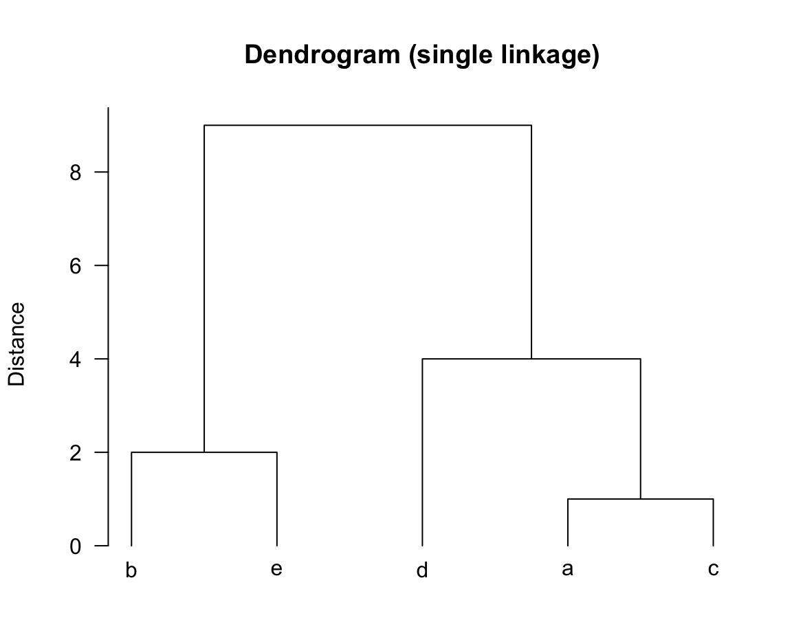
In the image above, the horizontal axis is used to locate the objects, placing them in the way they are being clustered. In turn, the vertical axis shows the distance index. As you can tell, the first cluster \(\textsf{ac}\) is has a distance of 1. The cluster \(\textsf{be}\) has a distance of 2, and so on and so forth.
32.3 Example: Complete Linkage
In complete linkage, we look at the pair of objects that are farthest apart.
We start again with the set of \(n=5\) objects, and the matrix of squared Euclidean distances:
Figure 32.11: Five objects and their distances
The first step is the same as in single linkage, that is, we look for the pair of points with the closest distance which we is the pair \((\textsf{a}, \textsf{c})\). We now treat this pair as a single point, and recompute distances:
Figure 32.12: The two closest objects
We have now four objects: a cluster \(\textsf{ac}\), and three individuals
\(\textsf{b}\), \(\textsf{d}\), and \(\textsf{e}\).
We know that the distance between \(\textsf{b}\) and \(\textsf{d}\) is 25. Also,
the distance between \(\textsf{b}\) and \(\textsf{e}\) is 2. But what about
the distance between cluster \(\textsf{ac}\) and \(\textsf{b}\)? How do we determine
the distance between a cluster and a point?
Figure 32.13: Distance between a cluster and other objects?
In complete linkage we define the distance between the cluster \((\textsf{ac})\) and individual \(\textsf{b}\) to be:
\[ d^2(\textsf{ac}, \textsf{b}) = max \{ d^2(\textsf{a},\textsf{b}), \hspace{2mm} d^2(\textsf{c},\textsf{b}) \} \]
For example, in our toy dataset we have:
- \(d^2(\textsf{ac}, \textsf{b}) = \max\{16, 17\} = 17\)
- \(d^2(\textsf{ac}, \textsf{d}) = \max\{9, 4\} = 9\)
- \(d^2(\textsf{ac}, \textsf{e}) = \max\{10, 9\} = 10\)

Figure 32.14: Aggregation Criteria in Complete Linkage
Once we have the distances, we look for the next pair of objects that are closest to each other. In this case, those objects are \(\textsf{b}\) and \(\textsf{e}\).

Figure 32.15: Second cluster
So now we have two clusters \(\textsf{ac}\) and \(\textsf{be}\), and a third individual object \(\textsf{d}\). The matrix of distances is updated as follows:

Figure 32.16: Updating distances between clusters and objects
We then select the smallest distance which corresponds to the distance between cluster \(\textsf{ac}\) and individual \(\textsf{d}\):

Figure 32.17: Third cluster
And finally, after picking \(\textsf{acd}\), we get the last partition that groups all individuals into a unique cluster:

Figure 32.18: Three partitions
So, in this case our final grouping did not differ from that obtained using single linkage; the only difference will be our dendrogram:
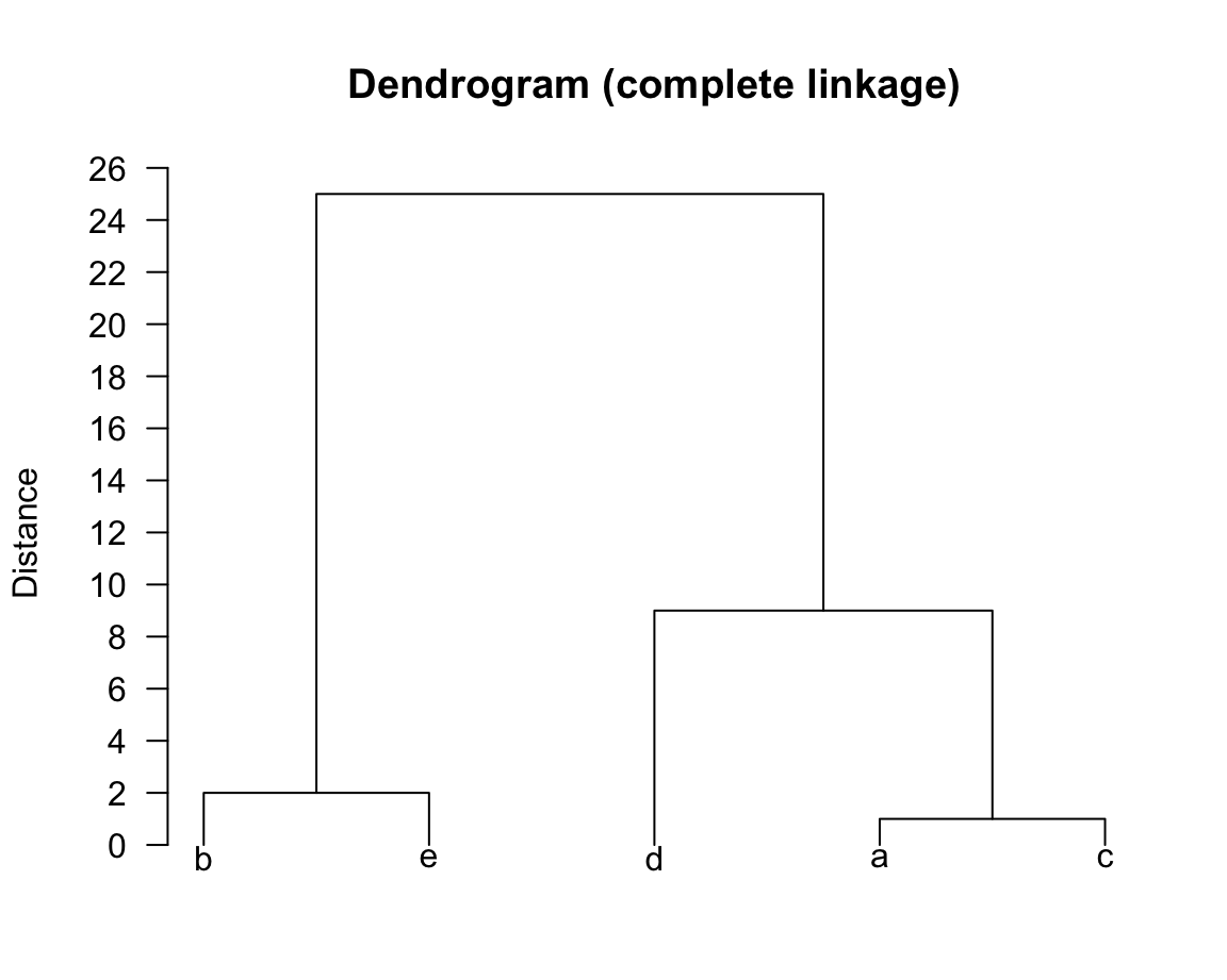
32.3.1 Cutting Dendograms
Depending on where we cut our dendrogram, we get different number of groups. For example, in our second dendrogram above, if we cut it at the value 20 we would obtain two clusters: \((\textsf{a}, \textsf{c}, \textsf{d})\) and \((\textsf{b}, \textsf{e})\).
Note that in this way, we can interpret the vertical distance on a dendrogram as a sort of measure for how stable our clusters are. For illustrative purposes, consider the dendrogram from complete linkage: after grouping \((\textsf{ac})\) with \(\textsf{d}\) (at a distance of 9), the algorithm did not produce any more groups until we reached a distance of 20. In this way, we might suspect that \(K = 3\) is a good guess for the true number of groups.
What Could Go Wrong
For example, what could go wrong with complete linkage? Well, outliers. In the presence of outliers, complete linkage will favor these points and this could mess with our results severely.
Note that both \(k-\)means and hierarchical clustering require notions of distances, even though those notions may be drastically different.
32.3.2 Pros and COons
Agglomerative methods:
- Have quadratic cost
- The dendrogram provides information about the whole process of aggregation
- A dendrogram also gives clue about the number of clusters
Direct partitioning methods:
- Have linear cost
- Number of groups must be predetermined
- Local optimal partition
We can take advantage of both approaches:
- Perform hierarchical clustering
- Determine the number of groups
- Calculate the corresponding centroids
- Perform K-means using as seeds the centroids previously calculated
What about clustering very large data sets?
- Perform \(m\) = 2 or 3 times a K-means algorithm (with \(K\) = 10)
- Form the crosstable of the \(m\) obtained partitions
- Calculate the centroids of the non-empty cells of the crosstable
- Perform hierarchical clustering of the centroids, weighed by the number of individuals per cell
- Determine the number of clusters
- Consolidate the clustering configuration