4 Principal Components Analysis
Our first unsupervised method of the book is Principal Components Analysis, commonly referred to as PCA.
Principal Components Analysis (PCA) is the workhorse method of multivariate data analysis. Simply put, PCA helps us study and explore a data set of quantitative variables measured on a set of objects. One way to look at the purpose of principal components analysis is to get the best low-dimensional representation of the variation in data. Among the various appealing features of PCA is that it allows us to obtain a visualization of the objects in order to see their proximities. Likewise, it also provides us results to get a graphic representation of the variables in terms of their correlations. Overall, PCA is a multivariate technique that allows us to summarize the systematic patterns of variations in a data set.
The classic reference for PCA is the work by the eminent British biostatistician Karl Pearson’s “On Lines and Planes of Closest Fit to Systems of Points in Space,” published in 1901. This publication presents the underlying problem of PCA from a purely geometric standpoint, describing how to find low-dimensional subspaces that best fit—in the least squares sense—a cloud of points. Keep in mind that Pearson never used the term principal components analysis. The other seminal work of PCA is the one by American mathematician and economic theorist Harold Hotelling with “Analysis of a Complex of Statistical Variables into Principal Components,” from 1933. It is Hotelling who coined the term principal components analysis and gave the method a more mature statistical perspective. Unlike Pearson, Hotelling finds the principal components as orthogonal linear combinations of the input variables in a way that such combinations have maximum variance.
PCA is one of those methods that can be approached from multiple, seemingly unrelated, perspectives. The way we are going to introduce PCA is not the typical way in which PCA is discussed in most books published in English. However, our introduction is actually based on the ideas and concepts originally published by Karl Pearson.
4.1 Low-dimensional Representations
Let’s play the following game. Imagine for a minute that you have the superpower to see any type of multidimensional space (not just three-dimensions). As we mentioned before, we think of the individuals as forming a cloud of points in a \(p\)-dim space, and the variables forming a cloud of arrows in an \(n\)-dim space.
Pretend that you have some data in which its cloud of points has the shape of a mug, like in the following diagram:

Figure 4.1: Cloud of points in the form of a mug
This mug is supposed to be high-dimensional, and something that you are not supposed to ever see in real life. So the question is: Is there a way in which we can get a low-dimensional representation of this data?
Luckily, the answer is: YES, we can!
How? Well, the name of the game is projections: we can look for projections of the data into sub-spaces of lower dimension, like in the diagram below.
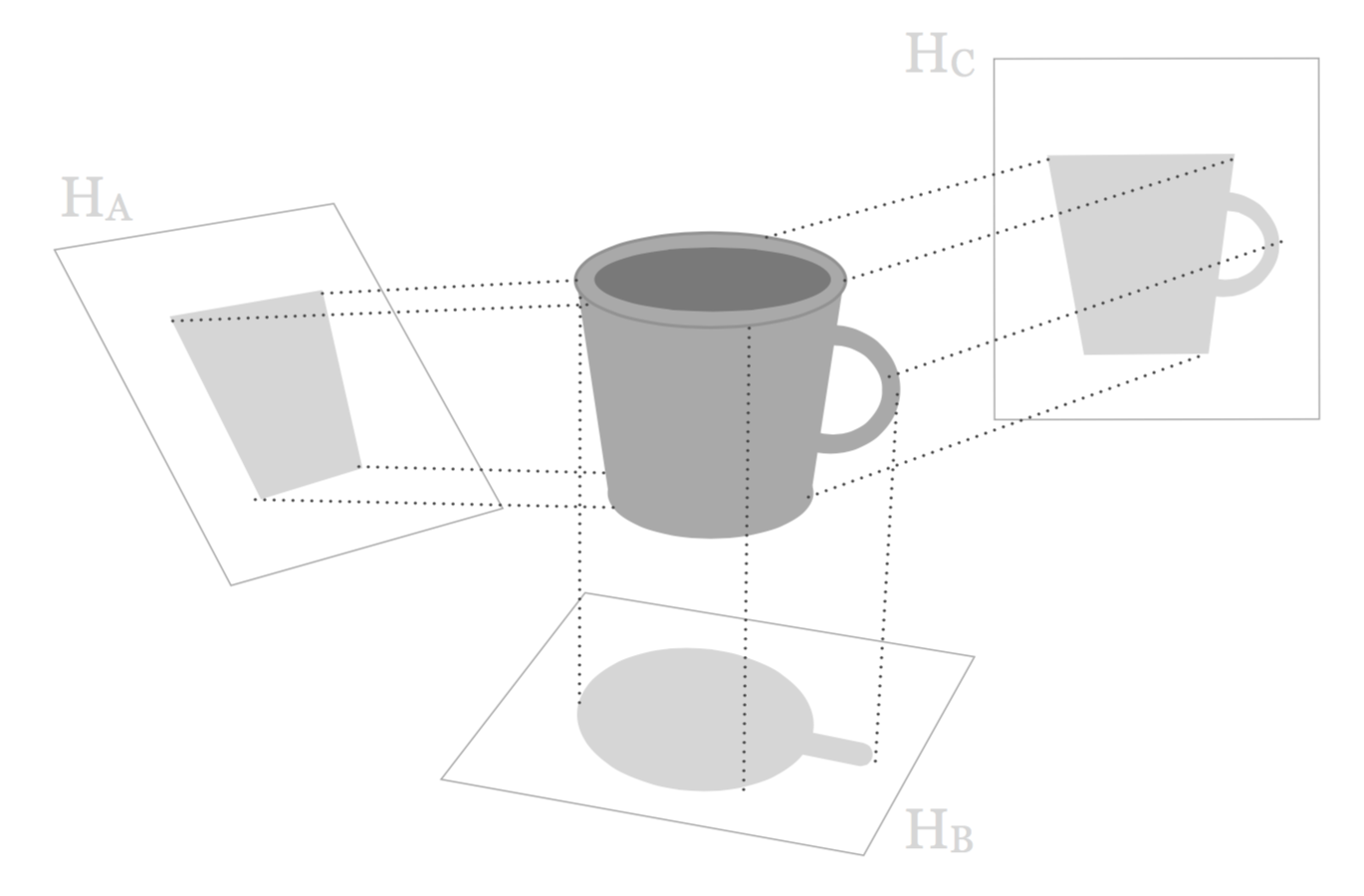
Figure 4.2: Various projections onto subspaces
Think of projections as taking photographs or x-rays of the mug. You can take a photo of the mug from different angles. For instance, you can take a picture in which the lens of the camera is on the top of the mug, or another picture in which the lens is below the mug (from the bottom), and so on.
If you have to take the “best” photograph of the mug, from what angle would you take such picture? To answer this question we need to be more precise about what do we mean by “best”. Here, we are talking about getting a picture in which the image of the mug is as similar as possible to the original object.
As you can tell from the above figure, we have three candidate subspaces: \(\mathbb{H}_A\), \(\mathbb{H}_B\), and \(\mathbb{H}_C\). Among the three possible projections, subspace \(\mathbb{H}_C\) is the one that provides the best low dimensional representation, in the sense that the projected silhouette is the most similar to the original mug shape.
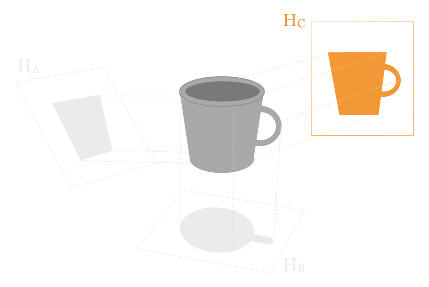
Figure 4.3: The shape of the projection is similar to the original mug shape.
We can say that the “photo” from projecting onto subspace \(\mathbb{H}_C\) is the one that most resembles the original object. Now, keep in mind that the resulting image in the low-dimensional space is not capturing the whole pattern. In other words, there is some loss of information. However, by choosing the right projection, we hope to minimize such loss.
4.2 Projections
Following the idea of projections, let’s now discuss with more detail this concept, and its implications.
Pretend that we zoom in to see some of the individuals of the cloud of points that form the mug (see figure below). Keep in mind that these data points are in a \(p\)-dimensional space, and the cloud will have its centroid \(\mathbf{g}\) (i.e. average individual).

Figure 4.4: Set of individuals in p-dim space.
Because our goal is to look for a low-dimensional represention, we can start by considering the simplest type of low-dimensional representations: a one-dimensional space. This in turn can be graphically displayed as one axis. In the above diagram (as well as the one below) this dimension is depicted with the yellow line, labeled as \(dim_{\mathbf{v}}\).

Figure 4.5: Set of individuals in p-dim space.
We should note that we don’t really manipulate dimension \(dim_{\mathbf{v}}\) directly. Instead, what we manipulate is a vector \(\mathbf{v}\) along this dimension.

Figure 4.6: Dimension spanned by vector v
At the end of the day, we want to project the individuals onto this dimension. In particular, the type of projections that we are interested in are orthogonal projections.

Figure 4.7: Projections onto one dimension
4.2.1 Vector and Scalar Projections
Let’s consider a specific individual, for example the \(i\)-th individual. And let’s take the centroid \(\mathbf{g}\) as the origin of the cloud of points. In this way, the dimension that we are looking for has to pass through the centroid of this cloud. Obtaining the orthogonal projection of the \(i\)-th individual onto the dimension \(dim_{\mathbf{v}}\) involves projecting \(\mathbf{x_i}\) onto any vector \(\mathbf{v}\) along this dimension.

Figure 4.8: Projection of an individual onto one dimension
Recall that an orthogonal projection can be split into two types of projections: (1) the vector projection, and (2) the scalar projection.
The vector projection of \(\mathbf{x_i}\) onto the \(\mathbf{v}\) is defined as:
\[ proj_{\mathbf{v}} (\mathbf{x_i}) = \frac{\mathbf{x_{i}^\mathsf{T} v}}{\mathbf{v^\mathsf{T}v}} \hspace{1mm} \mathbf{v} = \mathbf{\hat{v}} \tag{4.1} \]
The scalar projection of \(\mathbf{x_i}\) onto \(\mathbf{v}\) is defined as:
\[ comp_{\mathbf{v}} (\mathbf{x_i}) = \frac{\mathbf{x_{i}^\mathsf{T}v}}{\|\mathbf{v}\|} = z_{ik} \tag{4.2} \]
The following diagram displays both types of projections:

Figure 4.9: Scalar and vector projections of i-th individual onto vector v
We are not really interested in obtaining the vector projection \(proj_{\mathbf{v}} (\mathbf{x_i})\). Instead, what we care about is the scalar projection \(comp_{\mathbf{v}} (\mathbf{x_i})\). In other words, we just want to obtain the coordinate of the \(i\)-th individual along this axis.
4.2.2 Projected Inertia
As we said before, our goal is to find the angle that gives us the “best” photo of the mug (i.e. cloud of points). This can be translated as finding a subspace in which the distances between the points are most similar to those on the actual mug.

Figure 4.10: Projection Goal
Now, we need to define what we mean by “similar” distances in \(\mathbb{H}\). Consider the overall dispersion of our original system (the one with all \(p\) dimensions): \(\sum_{i} \sum_{\ell} d^2 (i, \ell)\). This is a fixed number; and we cannot change it. However, we can try fine-tune our subset \(\mathbb{H}\) such that:
\[ \sum_{i} \sum_{\ell} d^2 (i, \ell) \approx \sum_{i} \sum_{\ell} d_{\mathbb{H}}^2(i, \ell) \tag{4.3} \]
In the previous chapter, we learned about the so-called measure of “Overall Dispersion” which is basically the sum of all pairwise squared distances, which can also be expressed in terms of a sum of squared distances to the centroid:
\[ \sum_{i} \sum_{\ell} d^2 (i, \ell) = \ 2n \sum_i d^2 (i, g) \tag{4.4} \]
However, it will be easier to simply consider the inertia of the system (as opposed to the overall dispersion).
\[ 2n \sum_i d^2 (i, g) \ \longrightarrow \ \frac{1}{n} \sum_{i=1}^{n} d^2 (i, g) = \text{Inertia} \tag{4.5} \]
In mathematical terms, finding the subspace \(\mathbb{H}\) that gives us “similar” distances to those of the original space corresponds to maximizing the projected inertia:
\[ \max_{\mathbb{H}} \left\{ \frac{1}{n} \sum_{i=1}^{n} d_{\mathbb{H}}^2 (i, g) \right\} \tag{4.6} \]
Now, as we discuss before, the simplest subspace will be one dimension, that is, we consider the case where \(\mathbb{H} \subseteq \mathbb{R}^1\). So the first approach is to project our data points onto a vector \(\mathbf{v}\). Hence, the projected inertia becomes:
\[ \frac{1}{n} \sum_{i=1}^{n} d_\mathbb{H}^2 (i, g) = \frac{1}{n} \sum_{i=1}^{n} \left( \mathbf{x_i}^\mathsf{T} \mathbf{v} \right)^2 = \frac{1}{n} \sum_{i=1}^{n} z_i^2 \tag{4.7} \]
and our maximization problem becomes
\[ \max_{\mathbf{v}} \left\{ \frac{1}{n} \sum_{i=1}^{n} \left( \mathbf{x_i}^\mathsf{T} \mathbf{v} \right)^2 \right\} \quad \mathrm{s.t.} \quad \mathbf{v}^\mathsf{T} \mathbf{v} = 1 \tag{4.8} \]
For convenience, we add the restriction that \(\mathbf{v}\) is a unit-vector (vector of unit norm). Why do we need the constraint? If we didn’t have the constraint, we could always find a \(\mathbf{v}\) that obtains higher inertia, and things would explode. Furthermore, as we will see in the next section, this helps in the algebra we will use when we actually perform the maximization.
4.3 Maximization Problem
We now need to compute the projected Inertia. Without loss of generality, we will assume that we have mean-centered data. This implies that the centroid \(g\) of the cloud of points is now the origin \(g = 0\). Since we are projecting onto a line spanned by a unit-vector \(\mathbf{v}\), the projected inertia \(I_{\mathbb{H}}\) will simply be the variance of the projected data points:
\[ I_{\mathbb{H}} = \frac{1}{n} \sum_{i=1}^{n} d_\mathbb{H}^2(i, 0) = \frac{1}{n} \sum_{i=1}^{n} z_i^2 \tag{4.9} \]
In vector-matrix notation we have the following expressions:
\[ \mathbf{z} := \begin{pmatrix} z_1 \\ z_2 \\ \vdots \\ z_n \\ \end{pmatrix} \ \Longrightarrow \ I_\mathbb{H} = \frac{1}{n} \mathbf{z}^\mathsf{T} \mathbf{z} = \frac{1}{n} \mathbf{v}^\mathsf{T} \mathbf{X}^\mathsf{T} \mathbf{X} \mathbf{v} \tag{4.10} \]
Hence, the maximization problem becomes
\[ \max_{\mathbf{v}} \left\{ \frac{1}{n} \mathbf{v}^\mathsf{T} \mathbf{X}^\mathsf{T} \mathbf{X} \mathbf{v} \right\} \qquad \text{s.t.} \qquad \mathbf{v}^\mathsf{T} \mathbf{v} = 1 \tag{4.11} \]
To solve this maximization problem, we utilize the method of Lagrange Multipliers. The lagrangian \(\mathcal{L}\) is given by:
\[ \mathcal{L} = \frac{1}{n} \mathbf{v}^\mathsf{T} \mathbf{X}^\mathsf{T} \mathbf{X} \mathbf{v} - \lambda \left( \mathbf{v}^\mathsf{T} \mathbf{v} - 1 \right) \tag{4.12} \]
Calculating the derivative of the lagrangian \(\mathcal{L}\) with respect to \(\mathbf{v}\), and equating to zero we get:
\[ \frac{\partial \mathcal{L}}{\partial \mathbf{v}} = \frac{2}{n} \mathbf{X}^\mathsf{T} \mathbf{X} \mathbf{v} - 2 \lambda \mathbf{v} = \mathbf{0} \tag{4.13} \]
Doing some algebra, we get:
\[ \underbrace{ \frac{1}{n} \mathbf{X}^\mathsf{T} \mathbf{X} }_{:= \mathbf{S} } \mathbf{v} = \lambda \mathbf{v} \quad \Rightarrow \quad \mathbf{S} \mathbf{v} = \lambda \mathbf{v} \tag{4.14} \]
That is, we obtain the equation \(\mathbf{S} \mathbf{v} = \lambda \mathbf{v}\) where \(\mathbf{S} \in \mathbb{R}^{p \times p}\) is symmetric. This means that \(\mathbf{v}\) is an eigenvector (with eigenvalue \(\lambda\)) of \(\mathbf{S}\). Moreover, \(\lambda\) is the value of the projected inertia \(I_\mathbb{H}\)—which is the thing that we want to maximize.
4.3.1 Eigenvectors of \(\mathbf{S}\)
Assume that \(\mathbf{X}\) has full rank (i.e. \(\mathrm{rank}(\mathbf{X}) = p\)). We then obtain \(p\) eigenvectors, which together form the matrix \(\mathbf{V}\):
\[ \mathbf{V} = \begin{bmatrix} \mathbf{v_1} & \mathbf{v_2} & \dots & \mathbf{v_k} & \dots & \mathbf{v_p} \\ \end{bmatrix} \tag{4.15} \]
We can also obtain \(\mathbf{\Lambda}_{p \times p} := \mathrm{diag}\left\{ \lambda_i \right\}_{i=1}^{n}\) (i.e. the matrix of eigenvalues): that is,
\[ \mathbf{\Lambda} = \begin{bmatrix} \lambda_1 & 0 & \dots & 0 \\ 0 & \lambda_2 & \dots & 0 \\ \vdots & \vdots & \ddots & \vdots \\ 0 & 0 & \dots & \lambda_p \\ \end{bmatrix} \tag{4.16} \]
Finally, we can also obtain the matrix \(\mathbf{Z}_{n \times p}\) which is the matrix consisting of the vectors \(\mathbf{z_i}\):
\[ \mathbf{Z} = \begin{bmatrix} \mathbf{z_1} & \mathbf{z_2} & \dots & \mathbf{z_k} & \dots & \mathbf{z_p} \\ \end{bmatrix} \tag{4.17} \]
The matrix of eigenvectors \(\mathbf{V}\) is known as the matrix of loadings (in PCA jargon)
The matrix of projected points \(\mathbf{Z}\) is known as the matrix of principal components (PC’s), also known as scores (in PCA jargon).
Let us examine the \(k\)-th principal component \(\mathbf{z_k}\):
\[ \mathbf{z_k} = \mathbf{X v_k} = v_{1k} \mathbf{x_1} + v_{2k} \mathbf{x_2} + \dots + v_{pk} \mathbf{x_p} \tag{4.18} \]
(where \(\mathbf{x_k}\) denotes columns of \(\mathbf{X}\)).
Note that \(\mathrm{mean}(\mathbf{z_k}) = 0\); since we are assuming that the data is mean-centered, we have that \(\mathrm{mean}(\mathbf{x_1}) = 0\).
What about variance of \(\mathbf{z_k}\)?
\[\begin{align*} Var(\mathbf{z_k}) & = \frac{1}{n} \mathbf{z_{k}^\mathsf{T}} \mathbf{z_k} \\ & = \frac{1}{n}\left( \mathbf{X} \mathbf{v_k} \right)^{\mathsf{T}} \left( \mathbf{X} \mathbf{v_k} \right) \\ & = \frac{1}{n} \mathbf{v_{k}^\mathsf{T}} \mathbf{X}^\mathsf{T} \mathbf{X} \mathbf{v_k} \\ & = \mathbf{v_k}^\mathsf{T} \mathbf{S} \mathbf{v_k} \\ & = \mathbf{v_k}^\mathsf{T} \left( \lambda_k \mathbf{v_k} \right) = \lambda_k \left( \mathbf{v_k}^\mathsf{T} \mathbf{v_k} \right) \\ & = \lambda_k \tag{4.19} \end{align*}\]
Hence, we obtain the following interesting result: the \(k\)-th eigenvalue of \(\mathbf{S}\) is simply the variance of the \(k\)-th principal component.
If \(\mathbf{X}\) is mean centered, then \(\mathbf{S} = \frac{1}{n} \mathbf{X^\mathsf{T} X}\) is nothing but the variance-covariance matrix of our data. If \(\mathbf{X}\) is standardized (i.e. mean-centered and scaled by the variance), then \(\mathbf{S}\) becomes the correlation matrix.
In summary:
\(\mathrm{mean}(\mathbf{z_k}) = 0\)
\(Var(\mathbf{z_k}) = \lambda_k\)
\(\mathrm{sd}(\mathbf{z_k}) = \sqrt{\lambda_k}\)
We have the following fact (the proof is omitted, and may be assigned as homework or as a test question):
\[ \text{Inertia} = \frac{1}{n} \sum_{i=1}^{n} d^2(i, g) = \sum_{k} \lambda_k = \mathrm{tr}\left( \frac{1}{n} \mathbf{X^\mathsf{T} X} \right) \tag{4.20} \]
The dimensions that we find in our analysis (through \(\mathbf{v_k}\)) relates directly to \(\mathbf{z_k}\).
\(\sum_{k=1}^{p} \lambda_k\) relates directly to the total amount of variability of our data.
Remark: The principal components capture different parts of the variability in the data.
4.4 Another Perspective of PCA
Having seen how to approach PCA from a geometric point of view, let us present another way to approach PCA from a variance maximazation standpoint, which is the most common way in which PCA is introduced within the Anglo-Saxon literature. Given a set of \(p\) variables \(\mathbf{x_1}, \mathbf{x_2}, \dots, \mathbf{x_p}\), we want to obtain new \(k\) variables \(\mathbf{z_1}, \mathbf{z_2}, \dots, \mathbf{z_k}\), called the Principal Components (PCs).
A principal component is a linear combination of the \(p\) variables: \(\mathbf{z} = \mathbf{Xv}\). The first PC is a linear mix which we graphically depict like this:

Figure 4.11: PCs as linear combinations of X-variables
The second PC is another linear mix:

Figure 4.12: PCs as linear combinations of X-variables
We want to compute the PCs as linear combinations of the original variables.
\[ \begin{array}{c} \mathbf{z_1} = v_{11} \mathbf{x_1} + \dots + v_{p1} \mathbf{x_p} \\ \mathbf{z_2} = v_{12} \mathbf{x_1} + \dots + v_{p2} \mathbf{x_p} \\ \vdots \\ \mathbf{z_k} = v_{1k} \mathbf{x_1} + \dots + v_{pk} \mathbf{x_p} \\ \end{array} \tag{4.21} \]
Or in matrix notation:
\[ \mathbf{Z} = \mathbf{X V} \tag{4.22} \]
where \(\mathbf{Z}\) is an \(n \times k\) matrix of principal components, and \(\mathbf{V}\) is a \(p \times k\) matrix of weights, also known as directional vectors of the principal axes. The following figure shows a graphical representation of a PCA problem in diagram notation:

Figure 4.13: PCs as linear combinations of X-variables
We look to transform the original variables into a smaller set of new variables, the Principal Components (PCs), that summarize the variation in data. The PCs are obtained as linear combinations (i.e. weighted sums) of the original variables. We look for PCs is in such a way that they have maximum variance, and being mutually orthogonal.
4.4.1 Finding Principal Components
The way to find principal components is to construct them as weighted sums of the original variables, looking to optimize some criterion and following some constraints. One way in which we can express the criterion is to require components \(\mathbf{z_1}, \mathbf{z_2}, \dots, \mathbf{z_k}\) that capture most of the variation in the data \(\mathbf{X}\). “Capturing most of the variation,” implies looking for a vector \(\mathbf{v_h}\) such that a component \(\mathbf{z_h} = \mathbf{X v_h}\) has maximum variance:
\[ \max_{\mathbf{v_h}} \; var(\mathbf{z_h}) \quad \Rightarrow \quad \max_{\mathbf{v_h}} \; var(\mathbf{X v_h}) \tag{4.23} \]
that is
\[ \max_{\mathbf{v_h}} \; \frac{1}{n} \mathbf{v_{h}^\mathsf{T} X^\mathsf{T} X v_h} \tag{4.24} \]
As you can tell, this is a maximization problem. Without any constraints, this problem is unbounded, not to mention useless. We could take \(\mathbf{v_h}\) as bigger as we want without being able to reach any maximum. To get a feasible solution we need to impose some kind of restriction. The standard adopted constraint is to require \(\mathbf{v_h}\) to be of unit norm:
\[ \| \mathbf{v_h} \| = 1 \; \hspace{1mm} \Rightarrow \; \hspace{1mm} \mathbf{v_{h}^\mathsf{T} v_h} = 1 \tag{4.25} \]
Note that \((1/n) \mathbf{X^\mathsf{T} X}\) is the variance-covariance matrix. If we denote \(\mathbf{S} = (1/n) \mathbf{X^\mathsf{T} X}\) then the criterion to be maximized is:
\[ \max_{\mathbf{v_h}} \; \mathbf{v_{h}^\mathsf{T} S v_h} \tag{4.26} \]
subject to \(\mathbf{v_{h}^\mathsf{T} v_h} = 1\)
To avoid a PC \(\mathbf{z_h}\) from capturing the same variation as other PCs \(\mathbf{z_l}\) (i.e. avoiding redundant information), we also require them to be mutually orthogonal so they are uncorrelated with each other. Formally, we impose the restriction \(\mathbf{z_h}\) to be perpendicular to other components: \(\mathbf{z_{h}^\mathsf{T} z_l} = 0; (h \neq l)\).
4.4.2 Finding the first PC
In order to get the first principal component \(\mathbf{z_1} = \mathbf{X v_1}\), we need to find \(\mathbf{v_1}\) such that:
\[ \max_{\mathbf{v_1}} \; \mathbf{v_{1}^\mathsf{T} S v_1} \tag{4.27} \]
subject to \(\mathbf{v_{1}^\mathsf{T} v_1} = 1\)
Being a maximization problem, the typical procedure to find the solution is by using the Lagrangian multiplier method. Using Lagrange multipliers we get:
\[ \mathcal{L} = \mathbf{v_{1}^\mathsf{T} S v_1} - \lambda (\mathbf{v_{1}^\mathsf{T} v_1} - 1) \tag{4.28} \]
Differentiation with respect to \(\mathbf{v_1}\), and equating to zero gives:
\[ \mathbf{S v_1} - \lambda_1 \mathbf{v_1} = \mathbf{0} \tag{4.29} \]
Rearranging some terms we get:
\[ \mathbf{S v_1} = \lambda_1 \mathbf{v_1} \tag{4.30} \]
What does this mean? It means that \(\lambda_1\) is an eigenvalue of \(\mathbf{S}\), and \(\mathbf{v_1}\) is the corresponding eigenvector.
4.4.3 Finding the second PC
In order to find the second principal component \(\mathbf{z_2} = \mathbf{X v_2}\), we need to find \(\mathbf{v_2}\) such that
\[ \max_{\mathbf{v_2}} \; \mathbf{v_{2}^\mathsf{T} S v_2} \tag{4.31} \]
subject to \(\| \mathbf{v_2} \| = 1\) and \(\mathbf{z_{1}^\mathsf{T} z_2} = 0\). Remember that \(\mathbf{z_2}\) must be uncorrelated to \(\mathbf{z_1}\). Applying the Lagrange multipliers, it can be shown that the desired \(\mathbf{v_2}\) is such that
\[ \mathbf{S v_2} = \lambda_2 \mathbf{v_2} \tag{4.32} \]
In other words. \(\lambda_2\) is an eigenvalue of \(\mathbf{S}\) and \(\mathbf{v_2}\) is the corresponding eigenvector.
4.4.4 Finding all PCs
All PCs can be found simultaneously by diagonalizing \(\mathbf{S}\). Diagonalizing \(\mathbf{S}\) involves expressing it as the product:
\[ \mathbf{S} = \mathbf{V \Lambda V^\mathsf{T}} \tag{4.33} \]
where:
- \(\mathbf{\Lambda}\) is a diagonal matrix
- the elements in the diagonal of \(\mathbf{\Lambda}\) are the eigenvalues of \(\mathbf{S}\)
- the columns of \(\mathbf{V}\) are orthonormal: \(\mathbf{V^\mathsf{T} V= I}\)
- the columns of \(\mathbf{V}\) are the eigenvectors of \(\mathbf{S}\)
- \(\mathbf{V^\mathsf{T}} = \mathbf{V^{-1}}\)
Diagonalizing a symmetric matrix is nothing more than obtaining its eigenvalue decomposition (a.k.a. spectral decomposition). A \(p \times p\) symmetric matrix \(\mathbf{S}\) has the following properties:
- \(\mathbf{S}\) has \(p\) real eigenvalues (counting multiplicities)
- the eigenvectors corresponding to different eigenvalues are orthogonal
- \(\mathbf{S}\) is orthogonally diagonalizable (\(\mathbf{S} = \mathbf{V \Lambda V^\mathsf{T}}\))
- the set of eigenvalues of \(\mathbf{S}\) is called the spectrum of \(\mathbf{S}\)
In summary: The PCA solution can be obtained with an Eigenvalue Decomposition of the matrix \(\mathbf{S} = (1/n) \mathbf{X^\mathsf{T}X}\)
4.5 Data Decomposition Model
Formally, PCA involves finding scores and loadings such that the data can be expressed as a product of two matrices:
\[ \underset{n \times p}{\mathbf{X}} = \underset{n \times r}{\mathbf{Z}} \underset{r \times p}{\mathbf{V^\mathsf{T}}} \tag{4.34} \]
where \(\mathbf{Z}\) is the matrix of PCs or scores, and \(\mathbf{V}\) is the matrix of loadings. We can obtain as many different eigenvalues as the rank of \(\mathbf{S}\) denoted by \(r\). Ideally, we expect \(r\) to be smaller than \(p\) so we get a convenient data reduction. But usually we will only retain just a few PCs (i.e. \(k \ll p\)) expecting not to lose too much information:
\[ \underset{n \times p}{\mathbf{X}} \approx \underset{n \times k}{\mathbf{Z}} \hspace{1mm} \underset{k \times p}{\mathbf{V^\mathsf{T}}} + \text{Residual} \tag{4.35} \]
The previous expression means that just a few PCs will optimally summarize the main structure of the data
4.5.1 Alternative Approaches
Finding \(\mathbf{z_h} = \mathbf{X v_h}\) with maximum variance has another important property that it is not always mentioned in multivariate textbooks but that we find worth mentioning. \(\mathbf{z_h}\) is such that
\[ \max \sum_{j = 1}^{p} cor^2(\mathbf{z_h, x_j}) \tag{4.36} \]
What this expression implies is that principal components \(\mathbf{z_h}\) are computed to be the best representants in terms of maximizing the sum of squared correlations with the variables \(\mathbf{x_1}, \mathbf{x_2}, \dots, \mathbf{x_p}\). Interestingly, you can think of PCs as predictors of the variables in \(\mathbf{X}\). Under this perspective, we can reverse the relations and see PCA from a regression-like model perspective:
\[ \mathbf{x_j} = v_{jh} \mathbf{z_h} + \mathbf{e_h} \tag{4.37} \]
Notice that the regression coefficient is the \(j\)-th element of the \(h\)-th eigenvector.