21 Nonparametric Regression
In this chapter we provide a high level intuition behind nonparametric regression procedures. Full disclaimer: most of what we talk about in the next chapters is going to center on the case when we have one predictor: \(p = 1\). We’ll make a couple of comments here and there about extensions to the multivariate case. But most things covered are for univariate regression. Why? Doing nonparametric regression in higher dimensions becomes very quickly statistically and computationally inefficient (e.g. curse of dimensionality).
21.1 Conditional Averages
Consider the following example that has to do with NBA players in the 2018 season. Specifically, we are looking at two variables: years of experience, and salary (in millions of dollars). Let’s assume that salary is the response \(Y\), and experience is the predictor \(X\). The image below depicts the scatterplot between \(X\) and \(Y\).
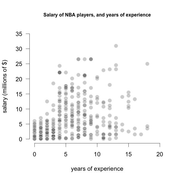
Figure 21.1: Salary -vs- Experience of NBA players
As you can tell, the relationship between Experience and Salary does not seem to be linear.
Say we are interested in predicting the salary for a player with four years of experience. One approach to get this prediction involves using a conditional mean:
\[ \text{Predicted Salary} = Avg(\text{Salary } | \text{ Experience = 4 years}) \]
A natural thing to do is to look at the salaries \(y_i\) of all players that have 4 years of experience: \(x_i = 4 \text{ years}\),
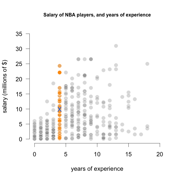
Figure 21.2: Salaries of players with 4 years of Experience
and then aggregate such salaries into a single value, for example, using the arithmetic mean:
\[ \hat{y}_0 = Avg(y_i | x_i = 4) \]
This is an empirical and nonparametric way to compute the conceptual definition of regression, which as we know, is defined in terms of conditional expectation:
\[ \textsf{regression function:} \quad \hat{f}(x_0) = \mathbb{E}(y | X = x_0) = \hat{y}_0 \]
We can compute all the average salaries for each value of years of experience, and make another plot with such averages:
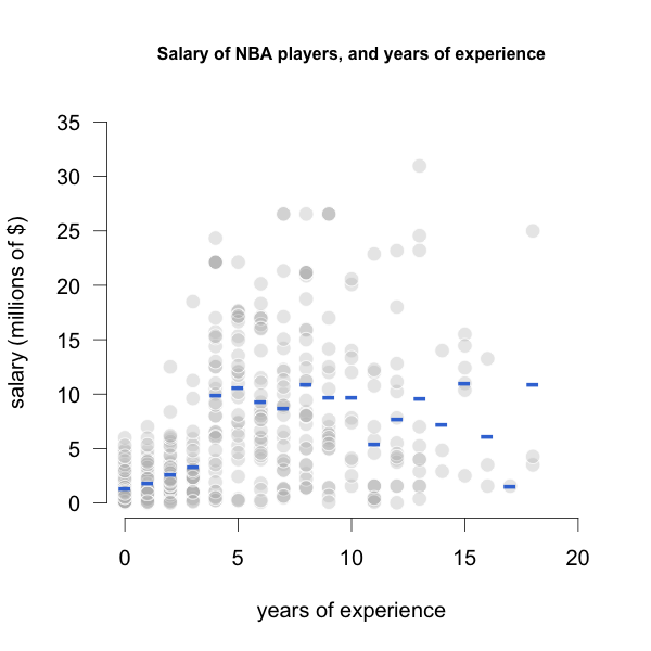
Figure 21.3: Average Salaries by years of Experience
Taking a further step, we can enrich the graph by connecting the dots of average salaries, in order to get a nonparametric regression line, displayed in the following image:
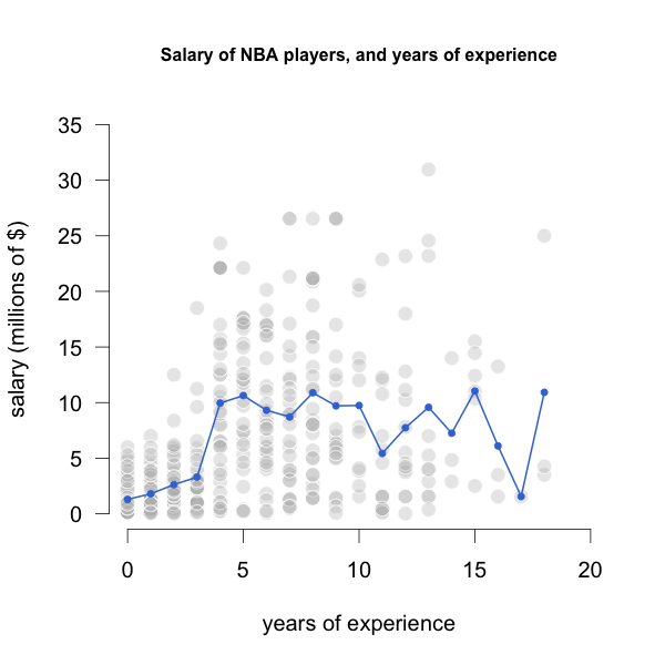
Figure 21.4: Average Salaries by years of Experience
Notice that this approach is surprisingly simple, and it does match the conceptual idea of regression as a conditional expectation. In this example, we are approximating such expectation with conditional averages: averages of salaries, conditioning by years of experience.
But this approach is not perfect. One of its downsides is that the fitted line looks very jagged. Another disadvantage is that we don’t have regression coefficients that helps us in the interpretation of the model.
In addition, we may have certain \(X\)-values for which there’s a scarcity of data. Consider for example the case of players with 17 years of experience in the NBA. The data from the 2018 season contains only one player with 17 years of experience. With just one data point, the predicted salary will be highly unreliable.
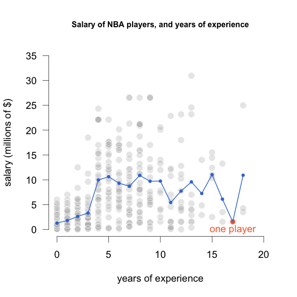
Figure 21.5: Only one player with 17 years of experience
21.2 Looking at the Neighbors
Because we only have one player with 17 years of experience, we need to find a way of using more of the data points in \(X\) to try to improve the prediction.
Looking at the scatterplot below, there are four players (the orange circles) that are very close to the player with 17 years of experience (red circle). So why not use the salaries of all these players to calculate a predicted salary for someone with 17 years of experience?
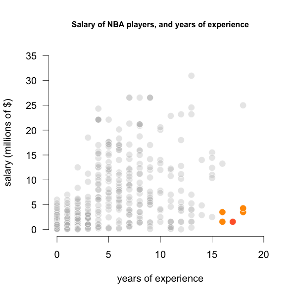
Figure 21.6: Four closest players to 17 years of experience
Some common options that we can use to profit from the neighboring data points are:
calculate the arithmetic mean of the neighboring \(y_i\)’s.
calculate a weighted average of the neighboring \(y_i\)’s.
calculate a linear fit with the neighboring \((x_i, y_i)\) points.
calculate a polynomial fit with the neighboring \((x_i, y_i)\) points.
Key Ideas
Let’s summarize what we have discussed so far with the following two core ideas:
Neighborhood: one of the main ideas has to do with the notion of neighboring points \(x_i\) for a given query point \(x_0\).
Local Fitting Mechanism: the other main idea implies some sort of mechanism to determine a local fit with the \(y_i\)’s (of the neighboring points) that we can use as the predicted outcome \(\hat{y_0}\).
In the next sections we describe a number of procedures that handle both of the above ideas in different ways, but that can be seen as special cases of what is known as linear smoothers.