35 Splitting Nodes
Having introduced the common measures of impurity in the previous chapter, let’s now review a fairly simple example by applying entropy and gini impurity indices on a two-class response classification problem.
Consider a simple credit data example, with 8 individuals described by three features (gender, job, region), and one response (status) with two categories: \(\text{good}\) and \(\text{bad}\) customers.
| gender | job | region | status | |
|---|---|---|---|---|
| a | male | yes | A | good |
| b | female | yes | B | good |
| c | male | no | C | good |
| d | female | yes | B | good |
| e | male | no | A | bad |
| f | female | no | B | bad |
| g | male | yes | C | bad |
| h | female | no | C | bad |
35.1 Entropy-based Splits
Let us encode \(\text{good}\) as a circle \(\bigcirc\), and let us encode \(\text{bad}\) as a square \(\square\). Our root node then contains 8 objects, with a 50-50 split in credit status:

Figure 35.1: Root node
Recall that the entropy of a particular node, \(H(\text{node})\), containing objects of \(k = 1, \dots, K\) classes, is given by:
\[ H(\text{node}) = - \sum_{k=1}^{K} p_k \log_2(p_k) \]
The entropy of the root node would therefore be
\[ H(\text{root}) = - \underbrace{ \frac{1}{2} \log_2\left( \frac{1}{2} \right) }_{\text{good}} - \underbrace{ \frac{1}{2} \log_2\left( \frac{1}{2} \right) }_{\text{bad}} = 1 \]
Partition by Gender
Now, say we choose to partition by gender. Our parent node would then split as follows:

Figure 35.2: Split by gender
Each of these child nodes have the same entropy:
\[ H(\text{left}) = - \underbrace{ \frac{1}{2} \log_2\left( \frac{1}{2} \right) }_{\text{good}} - \underbrace{ \frac{1}{2} \log_2\left( \frac{1}{2} \right) }_{\text{bad}} = 1 = H(\text{right}) \]
Now, we want to compare the combined entropies of these two child nodes and the entropy of the root node. That is, we compare
\[ H(\text{root}) \quad \text{-vs-} \quad \left( \frac{4}{8} \right) H(\text{left}) + \left( \frac{4}{8} \right) H(\text{right}) \]
Hence, let us define the information gain by the quantity
\[\begin{align*} \Delta I & = H(\text{root}) - \left[ \left( \frac{n_{\text{left}}}{n} \right) H(\text{left}) + \left( \frac{n_{\text{right}}}{n} \right) H(\text{right}) \right] \\ &= H(\text{root}) - \left[ \left( \frac{4}{8} \right) H(\text{left}) + \left( \frac{4}{8} \right) H(\text{right}) \right] \\ &= 1 - \left[ \frac{4}{8} + \frac{4}{8} \right] = 1 - 1 = 0 \end{align*}\]
In this way, we see that gender is not a good predictor to base our partitions on. Why? Because we obtain child nodes that have the same amount of entropy (the same amount of disorder) as the parent node.
Partition by Job
If we decide to partition by job, the parent node would then split as:

Figure 35.3: Split by job
The left node has an entropy of:
\[ H(\text{left}) = -\frac{3}{4} \log_2\left( \frac{3}{4} \right) -\frac{1}{4} \log_2\left( \frac{1}{4} \right) \approx 0.8112 \]
whereas the right node has an entropy of:
\[ H(\text{right}) = -\frac{1}{4} \log_2\left( \frac{1}{4} \right) -\frac{3}{4} \log_2\left( \frac{3}{4} \right) \approx 0.8112 \]
The information gain (i.e. reduction in impurity) \(\Delta I\) is thus:
\[\begin{align*} \Delta I &= H(\text{root}) - \frac{1}{2} H(\text{left}) - \frac{1}{2} H(\text{right}) \\ &= 1 - \frac{1}{2} (0.8112) - \frac{1}{2} (0.8112) \\ &\approx 0.1888 \end{align*}\]
Partition by Region
What about splitting the root node based on the categories of region? Note that region is a nominal qualitative variable with three categories, which means that there will be three possible binary partitions.

Figure 35.4: Splits by region
Region A -vs- Regions B,C
\[\begin{align*} \Delta I &= H(\text{root}) - \frac{2}{8} H(\text{left}) - \frac{6}{8} H(\text{right}) \\ &= 1 - \frac{2}{8} (1) - \frac{6}{8} (1) \\ &= 0 \end{align*}\]
Region B -vs- Regions A,C
\[\begin{align*} \Delta I &= H(\text{root}) - \frac{3}{8} H(\text{left}) - \frac{5}{8} H(\text{right}) \\ &= 1 - \frac{3}{8} (0.9183) - \frac{5}{8} (0.9709) \\ &\approx 0.0488 \end{align*}\]
Region C -vs- Regions A,B
\[\begin{align*} \Delta I &= H(\text{root}) - \frac{3}{8} H(\text{left}) - \frac{5}{8} H(\text{right}) \\ &= 1 - \frac{3}{8} (0.9183) - \frac{5}{8} (0.9709) \\ &\approx 0.04888 \end{align*}\]
Comparing the splits
As a summary, here are the following splits and the associated information gains:

We therefore see that splitting based on \(\text{Job}\) yields the best split (i.e. the split with the highest information gain).
In practice, this is the procedure that you would have to carry out. Try splitting based on all of the variables and compute the associated information gains, and visually ascertain which split results in the highest information gain. If there are ties in \(\Delta I\) values, it is customary to randomly select one to have a higher ranking than the other.
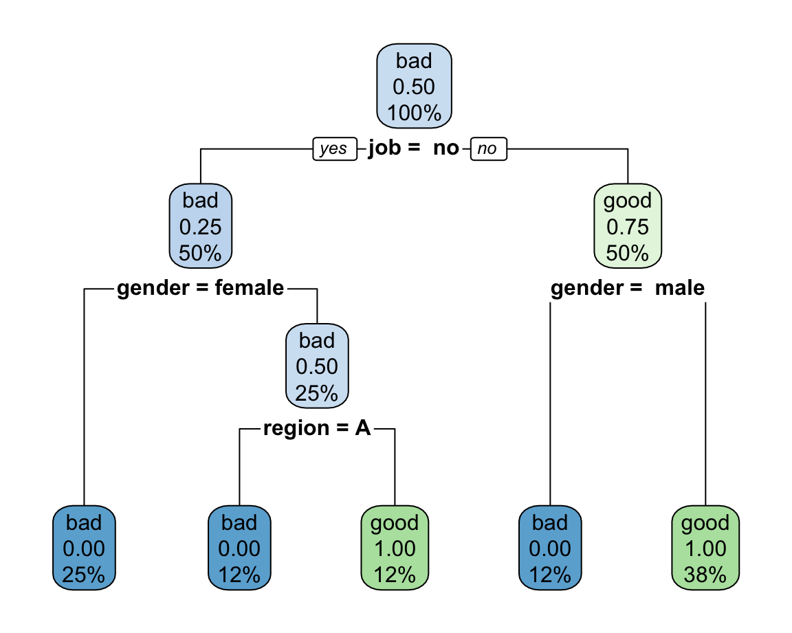
Entropy-based Classification Tree
The resulting classfication tree using entropy for binary splits is:
n= 8

node), split, n, loss, yval, (yprob)
      * denotes terminal node

 1) root 8 4 bad (0.5000000 0.5000000)
   2) job= no 4 1 bad (0.7500000 0.2500000)
     4) gender=female 2 0 bad (1.0000000 0.0000000) *
     5) gender=male 2 1 bad (0.5000000 0.5000000)
      10) region=A 1 0 bad (1.0000000 0.0000000) *
      11) region=C 1 0 good (0.0000000 1.0000000) *
   3) job=yes 4 1 good (0.2500000 0.7500000)
     6) gender= male 1 0 bad (1.0000000 0.0000000) *
     7) gender=female,male 3 0 good (0.0000000 1.0000000) *
with the tree diagram as follows:
35.2 Gini-index based Splits
Let’s repeat the same process but now calculating Gini impurities instead of entropies.
Recall that Gini impurity of a particular node, \(H(\text{node})\), containing objects of \(k = 1, \dots, K\) classes, is given by:
\[ Gini(\text{node}) = \sum_{k=1}^{K} p_k (1 - p_k) \]
Consider the root node:
Figure 35.5: Root node
The Gini impurity of the root node would therefore be:
\[\begin{align*} Gini(\text{root}) &= \sum_{k=1}^{2} p_k (1 - p_k) = \\ &= p_1(1-p_1) + p_2 (1 - p_2) \\ &= \frac{1}{2} \left(1 - \frac{1}{2} \right) + \frac{1}{2} \left( 1 - \frac{1}{2} \right) \\ &= 0.5 \end{align*}\]
Partition by Gender
We begin partitioning by gender. Our parent node would then split as follows:
Figure 35.6: Split by gender
Each of these child nodes have the same impurity:
\[\begin{align*} Gini(\text{left}) &= \sum_{k=1}^{2} p_k (1 - p_k) \\ &= \frac{1}{2} \left(1 - \frac{1}{2} \right) + \frac{1}{2} \left(1 - \frac{1}{2} \right) \\ &= \frac{1}{2} \cdot \frac{1}{2} + \frac{1}{2} \cdot \frac{1}{2} \\ &= 0.5 \\ &= Gini(\text{right}) \end{align*}\]
Now, we want to compare the combined entropies of these two child nodes and the entropy of the root node. That is, we compare
\[ Gini(\text{root}) \quad \text{-vs-} \quad \left( \frac{4}{8} \right) Gini(\text{left}) + \left( \frac{4}{8} \right) Gini(\text{right}) \]
Again, we use information gain defined by the quantity
\[\begin{align*} \Delta I & = Gini(\text{root}) - \left[ \left( \frac{n_{\text{left}}}{n} \right) Gini(\text{left}) + \left( \frac{n_{\text{right}}}{n} \right) Gini(\text{right}) \right] \\ &= Gini(\text{root}) - \left[ \left( \frac{4}{8} \right) Gini(\text{left}) + \left( \frac{4}{8} \right) Gini(\text{right}) \right] \\ &= 0.5 - \left[ \frac{4}{8} \cdot \frac{1}{2} + \frac{4}{8} \cdot \frac{1}{2} \right] = 0.5 - 0.5 = 0 \end{align*}\]
As you can tell, using Gini index, we obtain the same information \(\Delta I\) value as when using entropy on the gender-based split. Consequently, this feature is not a helpful predictor to base our partitions on.
Partition by Job
If we decide to partition by job, the parent node would then split as:
Figure 35.7: Split by job
The left node has a gini impurity of:
\[ Gini(\text{left}) = \frac{3}{4} \left(1- \frac{3}{4} \right) + \frac{1}{4} \left( 1 - \frac{1}{4} \right) = 0.375 \]
whereas the right node has a gini impurity of:
\[ Gini(\text{right}) = \frac{1}{4} \left( 1 - \frac{1}{4} \right) + \frac{3}{4} \left( 1 - \frac{3}{4} \right) = 0.375 \]
The information gain (i.e. reduction in impurity) \(\Delta I\) is thus:
\[\begin{align*} \Delta I &= Gini(\text{root}) - \frac{1}{2} Gini(\text{left}) - \frac{1}{2} Gini(\text{right}) \\ &= 0.5 - \frac{1}{2} (0.375) - \frac{1}{2} (0.375) \\ &= 0.125 \end{align*}\]
Partition by Region
Finally, let’s split the root node based on the categories of region.
Figure 35.8: Splits by region
Region A -vs- Regions B,C
\[\begin{align*} \Delta I &= Gini(\text{root}) - \frac{2}{8} Gini(\text{left}) - \frac{6}{8} Gini(\text{right}) \\ &= 0.5 - \frac{2}{8} (0.5) - \frac{6}{8} (0.5) \\ &= 0 \end{align*}\]
Region B -vs- Regions A,C
\[\begin{align*} \Delta I &= Gini(\text{root}) - \frac{3}{8} Gini(\text{left}) - \frac{5}{8} Gini(\text{right}) \\ &\approx 0.5 - \frac{3}{8} (0.4444) - \frac{5}{8} (0.48) \\ &\approx 0.0333 \end{align*}\]
Region C -vs- Regions A,B
\[\begin{align*} \Delta I &= Gini(\text{root}) - \frac{3}{8} Gini(\text{left}) - \frac{5}{8} Gini(\text{right}) \\ &\approx 0.5 - \frac{3}{8} (0.4444) - \frac{5}{8} (0.48) \\ &\approx 0.0333 \end{align*}\]
Comparing the splits
As a summary, here are the following splits and the associated information gains:

We therefore see that splitting based on \(\text{Job}\) yields the best split (i.e. the split with the highest information gain).
Gini-based Classification Tree
The resulting classfication tree using Gini-impurity for binary splits is:
n= 8

node), split, n, loss, yval, (yprob)
      * denotes terminal node

 1) root 8 4 bad (0.5000000 0.5000000)
   2) job= no 4 1 bad (0.7500000 0.2500000)
     4) gender=female 2 0 bad (1.0000000 0.0000000) *
     5) gender=male 2 1 bad (0.5000000 0.5000000)
      10) region=A 1 0 bad (1.0000000 0.0000000) *
      11) region=C 1 0 good (0.0000000 1.0000000) *
   3) job=yes 4 1 good (0.2500000 0.7500000)
     6) gender= male 1 0 bad (1.0000000 0.0000000) *
     7) gender=female,male 3 0 good (0.0000000 1.0000000) *
with the tree diagram as follows:

35.3 Looking for the best split
Let’s quickly review the steps for splitting a node, which involve the first two aspects listed above.
The main idea to grow a tree is to successively (i.e. recursively) divide the set of objects with the help of features \(X_1, \dots, X_p\), in order to obtain nodes that are as homogeneous as possible (with respect to the response).
Here’s what we have to do in a given (parent) node:
- Compute impurity of the (parent) node
- For each variable feature \(X_j\)
- Determine the number of binary splits
- For each binary split:
- compute impurity for left node
- compute impurity for right node
- calculate and store reduction in impurity (information gain)
- Find the best splitting feature \(X_j\) that has the maximum reduction in impurity.
Once you find the optimal split, perform the split, and repeat the above procedure for the new child nodes.