14 Regularization Techniques
In this part of the book we will talk about the notion of regularization (what is regularization, what is the purpose of regularization, what approaches are used for regularization) all of this within the context of linear models. However, keep in mind that you can also use regularization in non-linear contexts.
So what is regularization? If you look at the dictionary definition of the term regularization you should find something like this:
regularization; the act of bringing to uniformity; make (something) regular
Simply put: regularization has to do with “making things regular”.
But what about regularization in the context of supervised learning? What are the “irregular” things that need to be made “regular”? In order to answer this question, we will first motivate the discussion by looking at the simulation example used in chapter Overfitting, and then we will focus on the effects of having predictors with high multicollinearity.
14.1 Example: Regularity in Models
Let’s use the simulation example from chapter Overfitting.
We consider a target function with some noise given by the following expression:
\[ f(x) = sin(1 + x^2) + \varepsilon \tag{14.1} \]
with the input variable \(x\) in the interval \([0,1]\), and the noise term \(\varepsilon \sim N(\mu=0, \sigma=0.03)\).
The function of the signal, \(sin(1 + x^2)\), is depicted in the figure below. Keep in mind that in real life we will never have this knowledge.
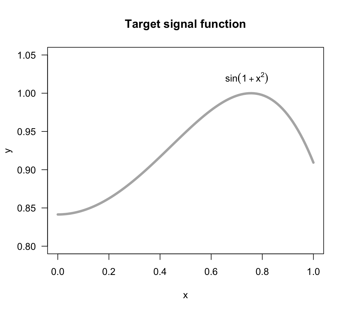
Figure 14.1: Target signal function
We randomly simulate seven in-sample sets each of size 10 points \((x_i, y_i)\); and for each set we fit several regression models using polynomials of various degrees from 1 to 9 (see figure below).
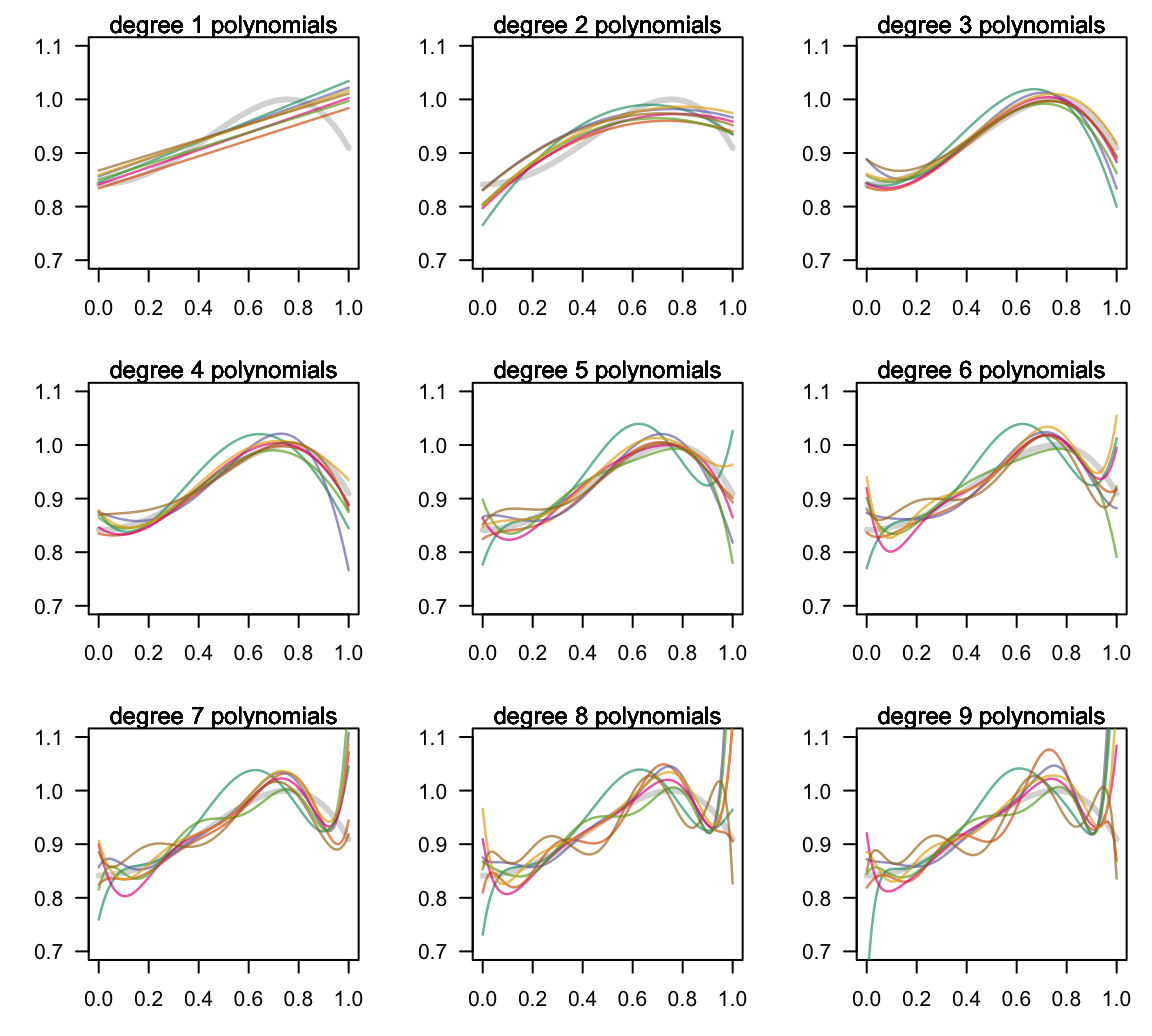
Figure 14.2: Fitting various polynomials of increasing complexity
Notice again the high flexibility of the high-order polynomials, namely those of degree 7, 8 and 9. These polynomials show an extremely volatile behavior. In contrast, the low-order polynomials (e.g. degrees 1 t o 3) are much more stable.
In general, we can say that the low-order polynomials are very “regular” because even though the data sets change for every fitted model, the obtained fits are fairly similar. Likewise, we can say that the mid-order polynomials of degrees 4-to-6 are somewhat “regular” with one or two data sets resulting in atypical fits compared to the rest. Finally, the high-order polynomials are very “irregular”; by this we mean that changing from one in-sample data set to another produces a remarkably different fit.
On one hand, we know that low-complexity models behave more regularly but they tend to have low learning capacity. Put in more formal terms: they tend to have small variance but at the expense of exhibiting large bias.
On the other hand, we also know that high-complexity models tend to have more learning capacity with a better opportunity to get closer to the target model. However, this increased capacity comes at the expense of larger variance. In other words, they tend to have low bias but at the expense of exhibiting a more irregular behavior.
In summary, the notion of regularization is tightly connected to the bias-variance tradeoff. The larger the variance of models, the more irregular they will be, and viceversa. What regularization pursuits is to find ways of controlling the behavior (i.e. the variance) of more flexible models in order to obtain lower generalization errors. How? By simplifying or reducing the flexibility of models in a manner that their variance goes down without sacrifing too much bias.
Having exposed the high-level intuition of regularization, let’s discuss one of the typical causes for having irregular behavior in linear regression models: multicollinearity.
14.2 Multicollinearity Issues
One of the issues when fitting regression models is due to multicollinearity: the condition that arises when two or more predictors are highly correlated.
How does this affect OLS regression?
When one or more predictors are linear combinations of other predictors, then \(\mathbf{X^\mathsf{T} X}\) is singular. This is known as exact collinearity. When this happens, there is no unique least squares estimate \(\mathbf{b}\).
A more challenging problem arises when \(\mathbf{X^\mathsf{T} X}\) is close but not exactly singular. This is usually referred to as near perfect collinearity or, more commonly, as multicollinearity. Why is this a problem? Because multicollinearity leads to imprecise (i.e. unstable, irregular) estimates \(\mathbf{b}\).
What are the typical causes of multicollinearity?
- One or more predictors are linear combinations of other predictors
- One or more predictors are almost perfect linear combinations of other predictors
- There are more predictors than observations \(p > n\)
14.2.1 Toy Example
To illustrate the issues of dealing with multicollinearity, let’s play with
mtcars, one of the built-in data sets in R.
mtcars[1:10, ]
#>                    mpg cyl  disp  hp drat    wt  qsec vs am gear carb
#> Mazda RX4         21.0   6 160.0 110 3.90 2.620 16.46  0  1    4    4
#> Mazda RX4 Wag     21.0   6 160.0 110 3.90 2.875 17.02  0  1    4    4
#> Datsun 710        22.8   4 108.0  93 3.85 2.320 18.61  1  1    4    1
#> Hornet 4 Drive    21.4   6 258.0 110 3.08 3.215 19.44  1  0    3    1
#> Hornet Sportabout 18.7   8 360.0 175 3.15 3.440 17.02  0  0    3    2
#> Valiant           18.1   6 225.0 105 2.76 3.460 20.22  1  0    3    1
#> Duster 360        14.3   8 360.0 245 3.21 3.570 15.84  0  0    3    4
#> Merc 240D         24.4   4 146.7  62 3.69 3.190 20.00  1  0    4    2
#> Merc 230          22.8   4 140.8  95 3.92 3.150 22.90  1  0    4    2
#> Merc 280          19.2   6 167.6 123 3.92 3.440 18.30  1  0    4    4
Let’s use mpg as response, and disp, hp, and wt as predictors.
# response
mpg <- mtcars$mpg

# predictors
disp <- mtcars$disp
hp <- mtcars$hp
wt <- mtcars$wt

# standardized predictors
X <- scale(cbind(disp, hp, wt))
Let’s inspect the correlation matrix given by the equation below, assuming the data matrix of predictors \(\mathbf{X}\) is mean-centered:
\[ \mathbf{R} = \frac{1}{n-1} \mathbf{X^\mathsf{T} X} \tag{14.2} \]
# correlation matrix
cor(X)
#> disp hp wt
#> disp 1.0000000 0.7909486 0.8879799
#> hp 0.7909486 1.0000000 0.6587479
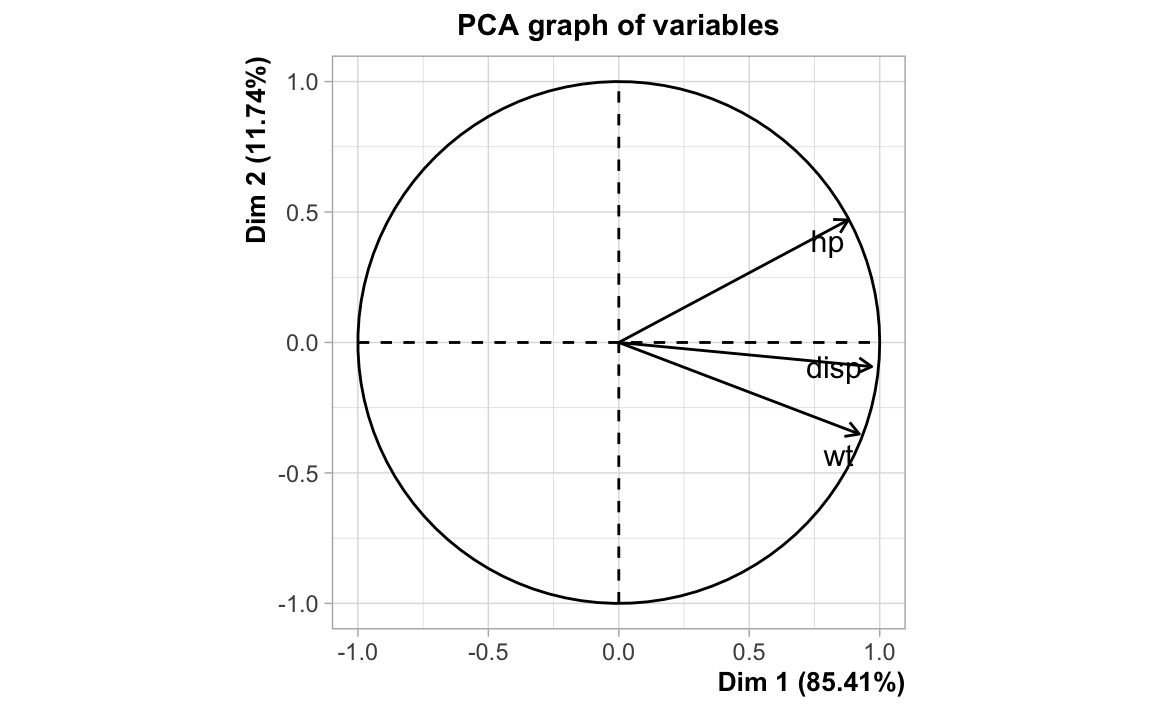
#> wt 0.8879799 0.6587479 1.0000000If we look at the circle of correlations from a principal components analysis,
we see the following pattern: hp, disp, and wt are positively correlated;
indicated by the fact the arrows are pointing in a common general direction.
Carrying out an ordinary least squares regression, that is, regressing mpg
onto disp, hp, and wt we get the following output provided the
linear model function lm():
#>
#> Call:
#> lm(formula = mpg ~ disp + hp + wt)
#>
#> Coefficients:
#> (Intercept)         disp           hp           wt
#>   37.105505    -0.000937    -0.031157    -3.800891
#>
#> Call:
#> lm(formula = mpg ~ disp + hp + wt)
#>
#> Residuals:
#>    Min     1Q Median     3Q    Max
#> -3.891 -1.640 -0.172  1.061  5.861
#>
#> Coefficients:
#>              Estimate Std. Error t value Pr(>|t|)
#> (Intercept) 37.105505   2.110815  17.579  < 2e-16 ***
#> disp        -0.000937   0.010350  -0.091  0.92851
#> hp          -0.031157   0.011436  -2.724  0.01097 *
#> wt          -3.800891   1.066191  -3.565  0.00133 **
#> ---
#> Signif. codes:  0 '***' 0.001 '**' 0.01 '*' 0.05 '.' 0.1 ' ' 1
#>
#> Residual standard error: 2.639 on 28 degrees of freedom
#> Multiple R-squared:  0.8268, Adjusted R-squared:  0.8083
#> F-statistic: 44.57 on 3 and 28 DF,  p-value: 8.65e-11
Analytically, the estimated vector of coefficients \(\mathbf{b}\), and the predicted response \(\mathbf{\hat{y}}\) are obtained as:
\(\mathbf{b} = (\mathbf{X^\mathsf{T} X})^{-1} \mathbf{X^\mathsf{T} y}\)
\(\mathbf{\hat{y}} = \mathbf{X} (\mathbf{X^\mathsf{T} X})^{-1} \mathbf{X^\mathsf{T} y}\)
So let’s take a look at the matrix \((\mathbf{X^\mathsf{T} X})^{-1}\)
#>             disp          hp          wt
#> disp  0.23627475 -0.08598357 -0.15316573
#> hp   -0.08598357  0.08827847  0.01819843
#> wt   -0.15316573  0.01819843  0.15627798
Exact Collinearity
Let’s introduce exact collinearity. For example, let’s create a fourth variable
disp1 that is a multiple of disp, and then let’s add this variable to the
data matrix X. What happens if we try to compute the inverse of
\(\mathbf{X_{1}^\mathsf{T} X_1}\)?
disp1 <- 10 * disp

X1 <- scale(cbind(disp, disp1, hp, wt))

solve(t(X1) %*% X1)
#> Error in solve.default(t(X1) %*% X1): system is computationally singular: reciprocal condition number = 1.55757e-17
As you can tell, R detected perfect collinearity, and the computation of the inverse shows that the matrix \(\mathbf{X_{1}^\mathsf{T} X_1}\) is singular.
Near-Exact Collinearity
Let’s introduce near-exact collinearity by creating a new variable disp2
which is almost a clone of disp, and put everything together in a new
matrix X2:
set.seed(123)
disp2 <- disp + rnorm(length(disp))

X2 <- scale(cbind(disp, disp2, hp, wt))

solve(t(X2) %*% X2)
#>              disp       disp2          hp          wt
#> disp   588.167214 -590.721826  1.01055902  1.99383316
#> disp2 -590.721826  593.525960 -1.10174784 -2.15719062
#> hp       1.010559   -1.101748  0.09032362  0.02220277
#> wt       1.993833   -2.157191  0.02220277  0.16411837
In this case, R was able to invert the matrix \(\mathbf{X_{2}^\mathsf{T} X_2}\). How does this compare with \((\mathbf{X^\mathsf{T} X})^{-1}\)?
solve(t(X) %*% X)
#>             disp          hp          wt
#> disp  0.23627475 -0.08598357 -0.15316573
#> hp   -0.08598357  0.08827847  0.01819843
#> wt   -0.15316573  0.01819843  0.15627798
When we compare \((\mathbf{X^\mathsf{T} X})^{-1}\) against
\((\mathbf{X_{2}^\mathsf{T} X_2})^{-1}\), we see that the first entry in the
diagonal of both matrices (the entry associated to disp) are very different.
More Extreme Near-Exact Collinearity
Let’s make things even more extreme! What about increasing the amount of
near-exact collinearity by creating a new variable disp3
which is almost a perfect clone of disp? This time we put everything in a new matrixX3`:
set.seed(123)
disp3 <- disp + rnorm(length(disp), mean = 0, sd = 0.1)

X3 <- scale(cbind(disp, disp3, hp, wt))

cor(disp, disp3)
#> [1] 0.9999997
And to make things more interesting, let’s create one more matrix,
denoted X31, that is a copy of X3 but contains a tiny modification,
that in theory, would hardly have any effect:
# small changes may have a "butterfly" effect
disp31 <- disp3

# change just one observation
disp31[1] <- disp3[1] * 1.01

X31 <- scale(cbind(disp, disp31, hp, wt))

cor(disp, disp31)
#> [1] 0.9999973
When we calculate the inverse of both \(\mathbf{X}_{3}^\mathsf{T} \mathbf{X}_{3}\) and \(\mathbf{X}_{31}^\mathsf{T} \mathbf{X}_{31}\), something weird happens:
solve(t(X3) %*% X3)
#>               disp        disp3           hp           wt
#> disp   59175.36325 -59202.97211  10.91501090  21.38646548
#> disp3 -59202.97211  59230.83035 -11.00617104 -21.54976679
#> hp        10.91501    -11.00617   0.09032362   0.02220277
#> wt        21.38647    -21.54977   0.02220277   0.16411837

solve(t(X31) %*% X31)
#>                 disp        disp31          hp          wt
#> disp    5941.5946101 -5942.3977358  0.30661752  0.64947961
#> disp31 -5942.3977358  5943.4373181 -0.39266978 -0.80278577
#> hp         0.3066175    -0.3926698  0.08830442  0.01825147
#> wt         0.6494796    -0.8027858  0.01825147  0.15638642
This is what we may call a “butterfly effect.” By modifying just one cell in \(\mathbf{X}_{31}\) by adding a little amount of random noise, the inverses \((\mathbf{X}_{3}^\mathsf{T} \mathbf{X}_{3})^{-1}\) and \((\mathbf{X}_{31}^\mathsf{T} \mathbf{X}_{31})^{-1}\) have changed dramatically. Which illustrates some of the issues when dealing with matrices that are not technically singular, but have a large degree of multicollinearity.
For comparison purposes:
# using predictors in X
reg <- lm(mpg ~ disp + hp + wt)
reg$coefficients
#>   (Intercept)          disp            hp            wt
#> 37.1055052690 -0.0009370091 -0.0311565508 -3.8008905826

# using predictors in X
reg2 <- lm(mpg ~ disp + disp2 + hp + wt)
reg2$coefficients
#> (Intercept)        disp       disp2          hp          wt
#> 36.59121161  0.43074188 -0.43323471 -0.02970117 -3.60121209

# using predictors in X3
reg3 <- lm(mpg ~ disp +  disp3  + hp + wt)
reg3$coefficients
#> (Intercept)        disp       disp3          hp          wt
#> 36.59121161  4.32985428 -4.33234711 -0.02970117 -3.60121209

# using predictors in X31
reg31 <- lm(mpg ~ disp + disp31 + hp + wt)
reg31$coefficients
#> (Intercept)        disp      disp31          hp          wt
#> 37.19129692  2.02426582 -2.02580803 -0.03091464 -3.76623514
14.3 Irregular Coefficients
Another interesting thing to look at in linear regression—via OLS—, is the theoretical variance-covariance matrix of the regression coefficients, given by:
\[ Var(\mathbf{\boldsymbol{\hat{\beta}}}) = \ \begin{bmatrix} Var(\hat{\beta}_1) & Cov(\hat{\beta}_1, \hat{\beta}_2) & \cdots & Cov(\hat{\beta}_1, \hat{\beta}_p) \\ Cov(\hat{\beta}_2, \hat{\beta}_1) & Var(\hat{\beta}_2) & \cdots & Cov(\hat{\beta}_2, \hat{\beta}_p) \\ \vdots & & \ddots & \vdots \\ Cov(\hat{\beta}_p, \hat{\beta}_1) & Cov(\hat{\beta}_p, \hat{\beta}_2) & \cdots & Var(\hat{\beta}_p) \\ \end{bmatrix} \tag{14.3} \]
Doing some algebra, the matrix \(Var(\boldsymbol{\hat{\beta}})\) can be compactly expressed in matrix notation as:
\[ Var(\boldsymbol{\hat{\beta}}) = \sigma^2 (\mathbf{X^\mathsf{T} X})^{-1} \tag{14.4} \]
The variance of a particular coefficient \(\hat{\beta}_j\) is given by:
\[ Var(\hat{\beta}_j) = \sigma^2 \left [ (\mathbf{X^\mathsf{T} X})^{-1} \right ]_{jj} \tag{14.5} \]
where \(\left [ (\mathbf{X^\mathsf{T} X})^{-1} \right ]_{jj}\) is the \(j\)-th diagonal element of \((\mathbf{X^\mathsf{T} X})^{-1}\)
A couple of remarks:
- Recall again that we don’t know \(\sigma^2\). How can we find an estimator \(\hat{\sigma}^2\)?
- We don’t observe the error terms \(\boldsymbol{\varepsilon}\) but we do have the residuals \(\mathbf{e = y - \hat{y}}\)
- We also have the Residual Sum of Squares (RSS)
\[ \text{RSS} = \sum_{i=1}^{n} e_{i}^{2} = \sum_{i=1}^{n} (y_i - \hat{y}_i)^2 \tag{14.6} \]
Effect of Multicollinearity
Assuming standardized variables, \(\mathbf{X^\mathsf{T} X} = n \mathbf{R}\), it can be shown that:
\[ Var(\boldsymbol{\hat{\beta}}) = \sigma^2 \left ( \frac{\mathbf{R}^{-1}}{n} \right ) \tag{14.7} \]
and \(Var(\hat{\beta}_j)\) can then be expressed as:
\[ Var(\hat{\beta}_j) = \frac{\sigma^2}{n} [\mathbf{R}^{-1}]_{jj} \tag{14.8} \]
It turns out that:
\[ [\mathbf{R}^{-1}]_{jj} = \frac{1}{1 - R_{j}^{2}} \tag{14.9} \]
which is known as the Variance Inflation Factor or VIF. If \(R_{j}^{2}\) is close to 1, then VIF will be large, and so \(Var(\hat{\beta}_j)\) will also be large.
Let us write the eigenvalue decomposition of \(\mathbf{R}\) as:
\[ \mathbf{R} = \mathbf{V \boldsymbol{\Lambda} V^\mathsf{T}} \tag{14.10} \]
And then express \(\mathbf{R}^{-1}\) in terms of the above decomposition:
\[\begin{align} \mathbf{R}^{-1} &= (\mathbf{V \Lambda} \mathbf{V}^\mathsf{T})^{-1} \\ &= \mathbf{V} \mathbf{\Lambda}^{-1} \mathbf{V}^\mathsf{T} \\ &= \begin{bmatrix} \mid & \mid & & \mid \\ \mathbf{v_1} & \mathbf{v_2} & \dots & \mathbf{v_p} \\ \mid & \mid & & \mid \\ \end{bmatrix} \begin{pmatrix} \frac{1}{\lambda_1} & 0 & \dots & 0 \\ 0 & \frac{1}{\lambda_2} & \dots & 0 \\ \vdots & \vdots & \ddots & \vdots \\ 0 & 0 & \dots & \frac{1}{\lambda_p} \\ \end{pmatrix} \begin{bmatrix} - \mathbf{v^\mathsf{T}_1} - \\ - \mathbf{v^\mathsf{T}_2} - \\ \vdots \\ - \mathbf{v^\mathsf{T}_p} - \\ \end{bmatrix} \tag{14.11} \end{align}\]
In this way, we obtain a formula for \(V(\hat{\beta}_j)\) involving the eigenvectors and eigenvalues of \(\mathbf{R}\) (as well as \(\sigma^2 / n\)):
\[ V(\hat{\beta}_j) = \frac{1}{n} \left ( \frac{\sigma^2}{\lambda_1} v_{j1}^2 + \frac{\sigma^2}{\lambda_2} v_{j2}^2 + \dots + \frac{\sigma^2}{\lambda_p} v_{jp}^2 \right) = \frac{\sigma^2}{n} \sum_{\ell=1}^{p} \frac{1}{\lambda_\ell} v_{j \ell}^2 \tag{14.12} \]
where \(v_{j \ell}\) denotes the \(j\)-th entry of the \(\ell\) eigenvector.
\[ Var(\hat{\beta}_j) = \left ( \frac{\sigma^2}{n} \right ) \sum_{\ell=1}^{p} \frac{v^{2}_{j \ell}}{\lambda_\ell} \tag{14.13} \]
The block matrix diagram above is designed to help visualize how we got these \(v_{\ell j}^2\) terms. As you can tell, the variance of the estimators depends on the inverses of the eigenvalues of \(\mathbf{R}\).
This formula is useful in interpreting collinearity. If we have perfect collinearity, some of the eigenvalues of \((\mathbf{X}^\mathsf{T} \mathbf{X})^{-1}\) would be equal to 0. In the case of near-perfect collinearity, some eigenvalues will be very close to 0. That is, \(\frac{1}{\lambda_\ell}\) will be very large. Stated differently: if we have multicollinearity, our OLS coefficients will have large variance.
In summary:
- the standard errors of \(\hat{\beta}_j\) are inflated.
- the fit is unstable, and becomes very sensitive to small perturbations.
- small changes in \(Y\) can lead to large changes in the coefficients.
What would you do to overcome multicollinearity?
- Reduce number of predictors
- If \(p > n\), then try to get more observations (increase \(n\))
- Find an orthogonal basis for the predictors
- Impose constraints on the estimated coefficients
- A mix of some or all of the above?
- Other ideas?
14.4 Connection to Regularization
So how all of the previous discussion connects with regularization? Generally speaking, we know that regularization has to do with “making things regular.” So, if you think about it, regularization implies that something is irregular.
In the context of regression, what is it that is irregular? What are the things that we are interested in “making regular”?
Within linear regression, regularization means reducing the variability—and therefore the size—of the vector of predicted coefficients. What we have seen is that if there is multicollinearity, some of the elements of \(\mathbf{b}_{ols}\) will have high variance. In other words, the norm \(\| \mathbf{b}_{ols} \|\) will be very large. When this is the case, we say that the coefficients are irregular. Consequently, regularization involves finding ways to mitigate the effects of these irregular coefficients.
Regularization Metaphor
Here’s a metaphor that we like to use when talking about regularization and the issue with “irregular” coefficients. As you know, in OLS regression, we want to find parameters that give us a linear combination of our response variables.

Figure 14.3: Linear combination without constant term
Think of finding the parameters \(b_1, \dots, b_p\) as if you go “shopping” for parameters. We assume (initially) that we have a blank check, and can pick whatever parameters we can buy. No need to worry about about how much they cost. If we are not careful (if there’s high multicollinearity) we could end up spending quite a lot of money.
To have some sort of budgeting control, we use regularization. This is like imposing some sort of restriction on what coefficients we can buy. We could use penalized methods or we could also use dimension reduction methods.
In penalized methods, we explicitly impose a budget on how much money we can spend when buying parameters.
In dimension reduction, there are no explicit penalties, but we still impose a “cost” on the regressors that are highly collinear. We reduce the number of parameters that we can buy.
The approaches that we will study—in the next chapters—for achieving regularization are:
Dimension Reduction: Principal Components Regression (PCR), Partial Least Squares regression (PLSR)
Penalized Methods: Ridge Regression, Lasso regression.