15 Principal Components Regression
The first dimension reduction method that we will describe to regularize a model is Principal Components Regression (PCR).
15.1 Motivation Example
To introduce PCR we are going to use a subset of the “2004 New Car and Truck Data” curated by Roger W. Johnson using records from Kiplinger’s Personal Finance. You can find more information about this data in the following url:
http://jse.amstat.org/datasets/04cars.txt
The data file, cars2004.csv, is available in the following github repository:
https://github.com/allmodelsarewrong/data
The data set consists of 10 variables measured on 385 cars. Here’s what the first six rows (and ten columns) look like:
                              price engine cyl  hp city_mpg
Acura 3.5 RL 4dr              43755    3.5   6 225       18
Acura 3.5 RL w/Navigation 4dr 46100    3.5   6 225       18
Acura MDX                     36945    3.5   6 265       17
Acura NSX coupe 2dr manual S  89765    3.2   6 290       17
Acura RSX Type S 2dr          23820    2.0   4 200       24
Acura TL 4dr                  33195    3.2   6 270       20
                              hwy_mpg weight wheel length width
Acura 3.5 RL 4dr                   24   3880   115    197    72
Acura 3.5 RL w/Navigation 4dr      24   3893   115    197    72
Acura MDX                          23   4451   106    189    77
Acura NSX coupe 2dr manual S       24   3153   100    174    71
Acura RSX Type S 2dr               31   2778   101    172    68
Acura TL 4dr                       28   3575   108    186    72
In this example we take the variable price as the response, and the rest of
the columns as input or predictor variables:
engine: engine size (liters)cyl: number of cylindershp: horsepowercity_mpg: city miles per gallonhw_mpg: highway miles per gallonweight: weights (pounds)wheel: wheel base (inches)length: length (inches)width: width (inches)
The regression model is:
\[ \texttt{price} = b_0 + b_1 \texttt{cyl} + b_2 \texttt{hp} + \dots + b_9 \texttt{width} + \boldsymbol{\varepsilon} \tag{15.1} \]
For exploration purposes, let’s examine the matrix of correlations among all variables:
engine cyl hp city_mpg hwy_mpg weight wheel length width
price 0.6 0.654 0.836 -0.485 -0.469 0.476 0.204 0.210 0.314
engine 0.912 0.778 -0.706 -0.708 0.812 0.631 0.624 0.727
cyl 0.792 -0.670 -0.664 0.731 0.553 0.547 0.621
hp -0.672 -0.652 0.631 0.396 0.381 0.500
city_mpg 0.941 -0.736 -0.481 -0.468 -0.590
hwy_mpg -0.789 -0.455 -0.390 -0.585
weight 0.751 0.653 0.808
wheel 0.867 0.760
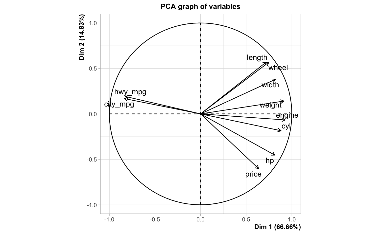
length 0.752And let’s also take a look at the circle of correlations, from the output of a PCA on the entire data set:
Computing the OLS solution for the regression model of price onto the
other nine predictors we obtain:
              Estimate  Std. Error  t value   Pr(>|t|)
(Intercept)  32536.025   17777.488   1.8302  6.802e-02
engine       -3273.053    1542.595  -2.1218  3.451e-02
cyl           2520.927     896.202   2.8129  5.168e-03
hp             246.595      13.201  18.6797  1.621e-55
city_mpg      -229.987     332.824  -0.6910  4.900e-01
hwy_mpg        979.967     345.558   2.8359  4.817e-03
weight           9.937       2.045   4.8584  1.741e-06
wheel         -695.392     172.896  -4.0220  6.980e-05
length          33.690      89.660   0.3758  7.073e-01
width         -635.382     306.344  -2.0741  3.875e-02
Out of curiosity, let’s compare the correlations—of the predictors and price—with the corresponding regression coefficients:
          correlation  coefficient
engine      0.5997873  -3273.05304
cyl         0.6544123   2520.92691
hp          0.8360930    246.59496
city_mpg   -0.4854130   -229.98735
hwy_mpg    -0.4694315    979.96656
weight      0.4760867      9.93652
wheel       0.2035464   -695.39157
length      0.2096682     33.69009
width       0.3135383   -635.38224
As you can tell from the above output, some correlation signs don’t match
the signs of their corresponding regression coefficients. For example,
engine is positively correlated with price but it turns out to have a
negative regression coefficient. Or look at hwy_mpg which is negatively
correlated with price but it has a positive regression coefficient.
15.2 The PCR Model
In PCR, like in PCA, we seek principal components \(\mathbf{z_1}, \mathbf{z_2}, \dots, \mathbf{z_r}\), linear combinations of the inputs: \(\mathbf{z_k} = \mathbf{Xv_k}\).

Figure 15.1: PCs as linear combinations of input variables
If we retain all principal components, then we know that we can factorize the input matrix \(\mathbf{X}\) as:
\[ \mathbf{X} = \mathbf{Z V^\mathsf{T}} \tag{15.2} \]
where:
- \(\mathbf{Z}\) is the matrix of principal components
- \(\mathbf{V}\) is the matrix of loadings
If we only keep a subset of \(k < p\) PCs, then we have a decomposition of the data matrix into a signal part captured by \(k\) components, and a residual or noise part:
\[ \underset{n \times p}{\mathbf{X}} = \underset{n \times k}{\mathbf{Z}} \hspace{1mm} \underset{k \times p}{\mathbf{V^\mathsf{T}}} + \underset{n \times p}{\mathbf{E}} \tag{15.3} \]

Figure 15.2: Matrix diagram for inputs
The idea is to use the components \(\mathbf{Z}\) as predictors of \(\mathbf{y}\). More specifically, the idea is to fit a linear regression in order to find coefficients \(\mathbf{b}\):
\[ \mathbf{y} = \mathbf{Zb} + \mathbf{e} \tag{15.4} \]

Figure 15.3: Matrix diagram for response
Usually, you don’t use all \(p\) PCs, but just a few of them. In other words, if we only keep a subset of \(k < p\) PCs, then the idea of PCR remains constant: use the \(k\) components in \(\mathbf{Z}\) as predictors of \(\mathbf{y}\):
\[ \mathbf{\hat{y}} = \mathbf{Z b} \tag{15.5} \]
Without loss of generality, suppose the predictors and response are standardized. In Principal Components Regression we regress \(\mathbf{y}\) onto the PC’s:
\[ \mathbf{\hat{y}} = b_1 \mathbf{z_1} + b_2 \mathbf{z_2} + \dots + b_k \mathbf{z_k} \tag{15.6} \]
The vector of PCR coefficients is obtained via ordinary least squares (OLS):
\[ \mathbf{b} = \mathbf{(Z^\mathsf{T} Z)^{-1} Z^\mathsf{T} y} \tag{15.7} \]
This is illustrated with the following diagram:

Figure 15.4: Path diagram of PCR
Using the cars2004 data set, with the PCA of the inputs, we can run a linear
regression of price onto all nine PCs:
Regression coefficients for all PCs
      Estimate  Std. Error   t value  Pr(>|t|)
PC1  -4470.761    205.1288  -21.7949    0.0000
PC2   7608.419    468.4759   16.2408    0.0000
PC3  -9650.324    660.1829  -14.6177    0.0000
PC4  -1768.547    980.6487   -1.8034    0.0721
PC5  10528.146   1115.0825    9.4416    0.0000
PC6  -5593.736   1177.6700   -4.7498    0.0000
PC7  -5746.452   1721.5725   -3.3379    0.0009
PC8  -7606.196   1926.3769   -3.9484    0.0001
PC9   5473.090   2660.3834    2.0573    0.0404
If we only take the first two PCs, the regression equation is
\[ \mathbf{\hat{y}} = b_1 \mathbf{z_1} + b_2 \mathbf{z_2} \tag{15.8} \]
and the regression coefficients are:
      Estimate  Std. Error   t value  Pr(>|t|)
PC1  -4470.761    205.1288  -21.7949         0
PC2   7608.419    468.4759   16.2408         0
Likewise, if take only the first three PCs, then the regression coefficients are:
      Estimate  Std. Error   t value  Pr(>|t|)
PC1  -4470.761    205.1288  -21.7949         0
PC2   7608.419    468.4759   16.2408         0
PC3  -9650.324    660.1829  -14.6177         0
Because of uncorrelatedness among principal components, the contributions and estimated coefficient of a PC are unaffected by which other PCs are also included in the regression.
15.3 How does PCR work?
Start with \(\mathbf{X} \in \mathbb{R}^{n \times p}\), assuming standardized data. Then, perform PCA on \(\mathbf{X}\): either an EVD of a multiple of \(\mathbf{X^\mathsf{T} X}\) (e.g. \((n-1)^{-1} \mathbf{X^\mathsf{T} X}\)), or the SVD of \(\mathbf{X} = \mathbf{U D V^\mathsf{T}}\). In either case, \(\mathbf{X} = \mathbf{Z V^\mathsf{T}}\) (the matrix of PC’s times the transpose of the matrix of loadings).
From OLS, we have:
\[ \mathbf{\hat{y}} = \mathbf{X (X^\mathsf{T} X)^{-1} X^\mathsf{T} y} = \mathbf{X} \mathbf{\overset{*}{b}} \tag{15.9} \]
Without loss of generality, let’s assume that \(\mathbf{X}\) is of full column rank \(p\). Assuming that we retain all principal components (\(k = p\)), then we can replace \(\mathbf{X}\) by \(\mathbf{Z V^\mathsf{T}}\) and therefore obtain:
\[\begin{align*} \mathbf{\hat{y}} &= \mathbf{X\overset{*}{b}}\\ &= \mathbf{X (X^\mathsf{T} X)^{-1} X^\mathsf{T} y} \\ &= \mathbf{Z V^\mathsf{T}} \left (\mathbf{(Z V^\mathsf{T})^\mathsf{T} Z V^\mathsf{T}} \right )^{-1} \mathbf{(Z V^\mathsf{T})^\mathsf{T} y} \\ &= \mathbf{Z V^\mathsf{T}} \left (\mathbf{V Z^\mathsf{T} Z V^\mathsf{T}} \right )^{-1} \mathbf{V Z^\mathsf{T} y} \\ &= \mathbf{Z V^\mathsf{T}} (\mathbf{V \Lambda V^\mathsf{T}})^{-1} \mathbf{V Z^\mathsf{T} y} \\ &= \mathbf{Z V^\mathsf{T}} (\mathbf{V} \mathbf{\Lambda}^{-1} \mathbf{V^\mathsf{T}}) \mathbf{V Z^\mathsf{T} y} \\ &= \mathbf{Z} \mathbf{\Lambda}^{-1} \mathbf{Z^\mathsf{T} y} \\ &= \mathbf{Zb^\text{pcr}} \tag{15.10} \end{align*}\]
15.3.1 Transition Formula
In PCR, if \(k = p\) (and assuming \(\mathbf{X}\) is of full-rank), which means that if you keep all PC’s, what happens is:
\[\begin{align*} \mathbf{\hat{y}} &= \mathbf{Z} \mathbf{b^\text{pcr}} \\ &= \mathbf{X V} \mathbf{b^\text{pcr}} \\ &= \mathbf{X} \mathbf{\overset{*}{b}} \tag{15.11} \end{align*}\]
In summary, when retaining all PC-scores \(k=p\), we can go back and forth between regression coefficients \(\mathbf{b^\text{pcr}}\), and regression coefficients \(\mathbf{\overset{*}{b}}\) for original input features, using the following transition equations:
\[ \mathbf{\overset{*}{b}} = \mathbf{V} \mathbf{b^\text{pcr}} \qquad \text{and} \qquad \mathbf{b^\text{pcr}} = \mathbf{V}^\mathsf{T} \mathbf{\overset{*}{b}} \tag{15.12} \]
Now, what if we decide to retain \(k < p\) PCs? Let \(\mathbf{Z_{1:k}}\) be the \(n \times k\) matrix with the first \(k\) PCs:
\[ \mathbf{Z_{1:k}} = [\mathbf{z_1}, \dots, \mathbf{z_k}] \tag{15.13} \]
and let \(\mathbf{b_{1:k}^\text{pcr}}\) be the corresponding vector of \(k\) regression coefficients such that:
\[ \mathbf{\hat{y}} = \mathbf{Z_{1:k}} \mathbf{b_{1:k}^\text{pcr}} \tag{15.14} \]
The good news is that we can still transition from \(Z\)-coefficients \(\mathbf{b_{1:k}^\text{pcr}}\) to \(X\)-coefficients \(\mathbf{X \overset{*}{b_k}}\), and viceversa.
\[ \mathbf{\hat{y}} = \mathbf{Z_{1:k}} \mathbf{b_{1:k}^\text{pcr}} = \mathbf{X V_{1:k}} \mathbf{b_{1:k}^\text{pcr}} = \mathbf{X \overset{*}{b_k}} \tag{15.15} \]
where \(\mathbf{\overset{*}{b_k}}\) is a vector of length equal to the number of columns in \(\mathbf{X}\); the subindex \(k\) indicates that it comes from the \(k\)-length vector \(\mathbf{b_{1:k}^\text{pcr}}\).
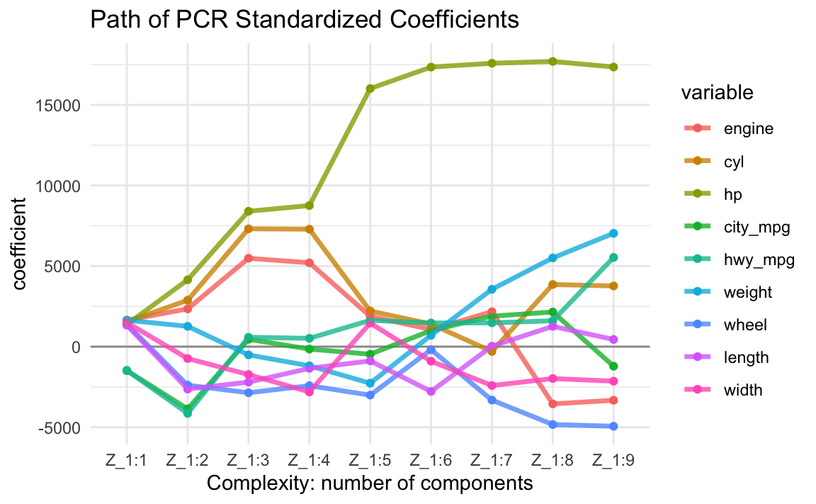
The following output shows the regression coefficients of all nine regression equations \(\mathbf{\hat{y}} = \mathbf{X \overset{*}{b_k}}\) in terms of the original input variables when we retain different number of components \(k=1, \dots, p\).
         Z_1:1 Z_1:2 Z_1:3 Z_1:4 Z_1:5 Z_1:6   Z_1:7 Z_1:8 Z_1:9
engine    1641  2345  5487  5203  1887  1064  2168.5 -3551 -3327
cyl       1544  2881  7312  7289  2213  1401  -295.5  3856  3766
hp        1377  4148  8402  8755 16016 17348 17585.7 17700 17352
city_mpg -1487 -3864   459  -149  -470   999  1891.3  2151 -1213
hwy_mpg  -1472 -4140   583   516  1633  1468  1477.9  1607  5536
weight    1642  1261  -510 -1187 -2266   707  3557.7  5507  7033
wheel     1385 -2392 -2860 -2422 -3009  -187 -3315.7 -4832 -4938
length    1332 -2634 -2202 -1346  -883 -2778    28.2  1260   447
width     1501  -738 -1731 -2811  1464  -904 -2413.8 -1978 -2142
For example, the values in the first column (column Z_1:1) are the regression
\(X\)-coefficients \(\mathbf{\overset{*}{b_1}}\) when using just the first PC.
\[ \mathbf{\hat{y}} = b_1^\text{pcr} \mathbf{z_1} = b_1^\text{pcr} \mathbf{Xv_1} = \mathbf{X} (b_1^\text{pcr} \mathbf{v_1}) = \mathbf{X} \mathbf{\overset{*}{b}_1} \tag{15.16} \]
The values in the second column (Z_1:2) are the \(X\)-coefficients
\(\mathbf{\overset{*}{b}_2}\) when using PC1 and PC2
\[ \mathbf{\hat{y}} = \mathbf{Z_{1:2}} \mathbf{b^\text{pcr}_{1:2}} = (\mathbf{X V_{1:2}}) \mathbf{b^\text{pcr}_{1:2}} = \mathbf{X} (\mathbf{V_{1:2}} \mathbf{b^\text{pcr}_{1:2}}) = \mathbf{X} \mathbf{\overset{*}{b}_{2}} \tag{15.17} \]
The values in the third column (Z_1:3) are the \(X\)-coefficients
\(\mathbf{\overset{*}{b}_{3}}\) when using PC1, PC2 and PC3; and so on.
Obviously, if you keep all components, you aren’t changing anything: “you’re spending the same amount of money as you were in regular least-squares regression”.
    engine        cyl         hp   city_mpg    hwy_mpg     weight      wheel
-3326.7904  3766.1495 17352.2185 -1213.0142  5535.9355  7032.5383 -4937.8106
    length      width
  446.9752 -2141.8196
compare with the regression coefficients of OLS:
   Xengine       Xcyl        Xhp  Xcity_mpg   Xhwy_mpg    Xweight     Xwheel
-3326.7904  3766.1495 17352.2185 -1213.0142  5535.9355  7032.5383 -4937.8106
   Xlength     Xwidth
  446.9752 -2141.8196
The idea is to keep only a few components. Hence, the goal is to find \(k\) principal components (with \(k \ll p\); \(k\) is called the tuning parameter or the hyperparameter). How do we determine \(k\)? The typical way is to use cross-validation.
15.3.2 Size of Coefficients
Let’s look at the evolution of the PCR derived coefficients \(\mathbf{\overset{*}{b}_{k}}\). This is a very interesting plot that allows us to see how the size of the coefficients grow as we add more and more PCs into the regression equation.
15.4 Selecting Number of PCs
The number \(k\) of PCs to use in PC Regression is a hyperparameter or tuning parameter. This means that we cannot derive an analytical expression that tells us what the number \(k\) of PCs is the optimal to be used. So how do we find \(k\)? We find \(k\) through resampling methods; the most popular resampling technique that most practioners apply is cross-validation, or other type of resampling approach. Here’s a description of the steps to be carried out.
Assumet that we have a training data set consisting of \(n\) data points: \(\mathcal{D}_{train} = (\mathbf{x_1}, y_1), \dots, (\mathbf{x_n}, y_n)\). To avoid confusion between the number of components \(k\), and the number of folds \(K\), here we are going to use \(Q = K\) to indicate the index of folds.
Using \(Q\)-fold cross-validation, we (randomly) split the data into \(Q\) folds:
\[ \mathcal{D}_{train} = \mathcal{D}_{fold-1} \cup \mathcal{D}_{fold-2} \dots \cup \mathcal{D}_{fold-Q} \]
Each fold set \(\mathcal{D}_{fold-q}\) will play the role of an evaluation set \(\mathcal{D}_{eval-q}\). Having defined \(Q\) fold sets, we form the corresponding \(Q\) retraining sets:
- \(\mathcal{D}_{train-1} = \mathcal{D}_{train} \setminus \mathcal{D}_{fold-1}\)
- \(\mathcal{D}_{train-2} = \mathcal{D}_{train} \setminus \mathcal{D}_{fold-2}\)
- \(\dots\)
- \(\mathcal{D}_{train-Q} = \mathcal{D}_{train} \setminus \mathcal{D}_{fold-Q}\)
The cross-validation procedure then repeats the following loop:
- For \(k = 1, 2, \dots, r = rank(\mathbf{X})\)
- For \(q = 1, \dots, Q\)
- fit PCR model \(h_{k,q}\) with \(k\)-PCs on \(\mathcal{D}_{train-q}\)
- compute and store \(E_{eval-q} (h_{k,q})\) using \(\mathcal{D}_{eval-q}\)
- end for \(q\)
- compute and store \(E_{cv_{k}} = \frac{1}{Q} \sum_k E_{eval-q}(h_{k,q})\)
- For \(q = 1, \dots, Q\)
- end for \(k\)
- Compare all cross-validation errors \(E_{cv_1}, E_{cv_2}, \dots, E_{cv_r}\) and choose the smallest of them, say \(E_{cv_{k^*}}\)
- Use \(k^*\) PCs to fit the (finalist) PCR model: \(\mathbf{\hat{y}} = b_1 \mathbf{z_1} + b_2 \mathbf{z_2} + \dots + b_{k^*} \mathbf{z_{k^*}} = \mathbf{Z_{1:k^*}} \mathbf{b_{1:k^*}}\)
- Remember that we can reexpress the PCR model in terms of the original predictors: \(\mathbf{\hat{y}} = (\mathbf{XV_{1:k^*}}) \mathbf{b_{1:k^*}} = \mathbf{X} \mathbf{\overset{*}{b}_k}\)
Remarks
The catch: those PC’s you choose to keep may not be good predictors of \(\mathbf{y}\). That is, there is a chance that some of those PC’s you discarded actually capture a fair amount of the signal. Unfortunately, there is no way of knowing this in a real-life setting. Partial Least Squares was developed as a cure for this, which is the topic of the next chapter.